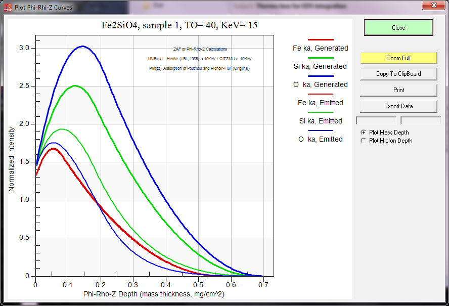
With Brian Joy's help we implemented prz plots for the PAP and XPP methods in CalcZAF v. 12.3.3. Here is a plot of the PAP curves for Fe2SiO4:
And here is the XPP plot:

As many of you know, the PAP prz method is interesting because it attempts to be physically accurate with regard to depth as opposed to other analytical models that focused primarily on the area under the curve (the genesis of PAP was thin film modeling by Pouchou). However, the validity of area under the curve analytical models is demonstrated by the surprising accuracy of the Love/Scott quadrilateral "prz" method which assumes the x-ray production distribution curve with depth is a rectangle! But since we're essentially comparing the ratio of the calculated intensity in a pure element with that of the compound, shape really doesn't matter.
Unless you really want to know the actual depth distribution of the x-ray production (e.g., a thin film). This is basically what I was getting at in this recent topic here:
http://probesoftware.com/smf/index.php?topic=1065.0Also, just as a reminder, the intensities plotted here are normalized intensities and only reflect the elements present, regardless of their concentrations. The only effect concentration has on the plotted intensities are seen in the emitted intensity curves due to the average mass absorption coefficients.
To demonstrate, here is a PAP model of TiO2 at 15 keV:

Here we can see that although oxygen x-rays are generated at a considerable depth, the O Ka x-ray emission volume is mostly within the top 200 nm of the sample. Download the latest CalcZAF 12.3.3 and try the same calculation but with the formula Ti99O or TiO99.


 Please keep your software updated for best results!