Following up on the trace carbon mapping topic here on the Probe Image board:
https://probesoftware.com/smf/index.php?topic=609.msg10167#msg10167Once probeman had properly acquired the X-ray maps in Probe Image, he proceeded to quantify the maps.
By the way, Probe Software is working on a new replicate X-ray map acquisition mode in Probe Image which will automatically acquire the replicate on-peak maps (for the TDI correction), and then once those on-peak replicates are acquired, it will automatically acquire the off-peak maps (if specified). This avoids any extra scans which would affect the carbon contamination rate. Obviously this is all moot if one is using the MAN background measurement method.
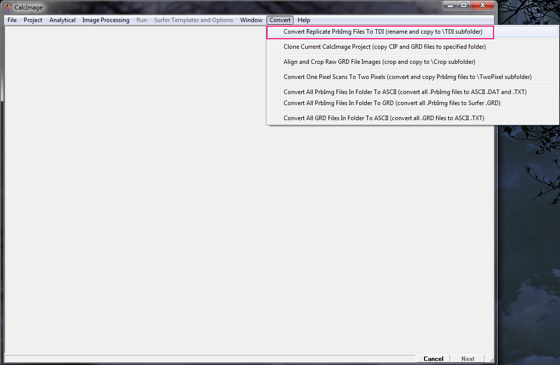
In the meantime, he first had to rename the replicate X-ray maps so that CalcImage knows these are intended for the TDI correction. That is done automatically using this Convert menu in CalcImage as shown here:
Once that is done he created a new project in CalcImage as usual by browsing to the /TDI sub folder and clicking on one map from each spectrometer pass. In this case the first pass for the 5 TDI elements and the second pass for the next 5 elements.
From the CalcImage Standard Assignments dialog we can now view the TDI intensities, here looking at carbon:
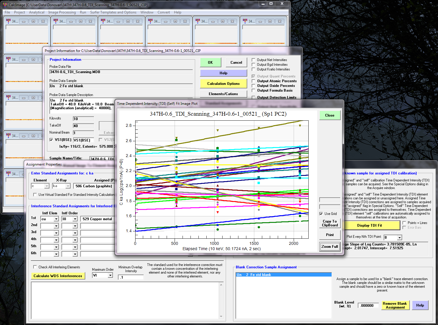
As we can see the intensity trend is slightly positive (using 5 2000 msec replicates over a total on-peak mapping time of about 40 minutes or so).
Please note that these maps were acquired with pixel dimensions of 116 x 2 pixels (X by Y) in order to more easily display the maps in Surfer which requires a minimum of 2 pixels in X and Y. Of course the JEOL stage would map in vertical direction so it would be 2 x 116 pixels (X by Y) in size for a JEOL stage map. Also note that one can convert one pixel tall (or wide) maps using the Convert | Convert One Pixel Scans To Two Pixels menu in CalcImage. This menu simply duplicates the 1 pixel dimension so the maps can be loaded into Surfer.
However, depending on the aspect ratio of the X-ray maps, one might need to adjust the displayed maps in Surfer. So after the maps are quantified and opened in Surfer, they might need to modify the X and Y proportions and Y axis length as shown here:
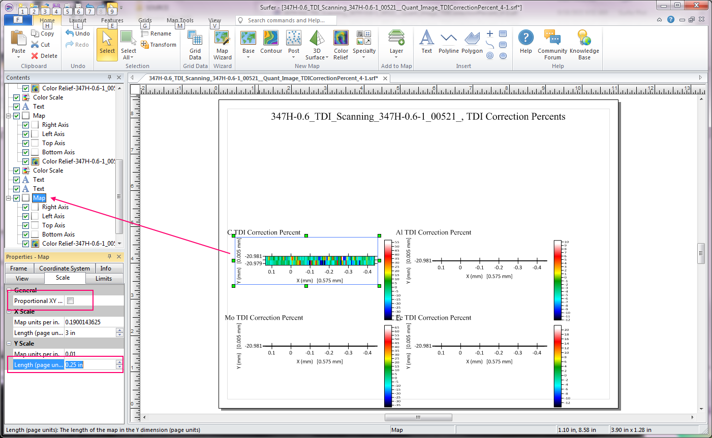
Here we are showing the TDI percent correction maps. Once all the axis lengths are adjusted we can see this:
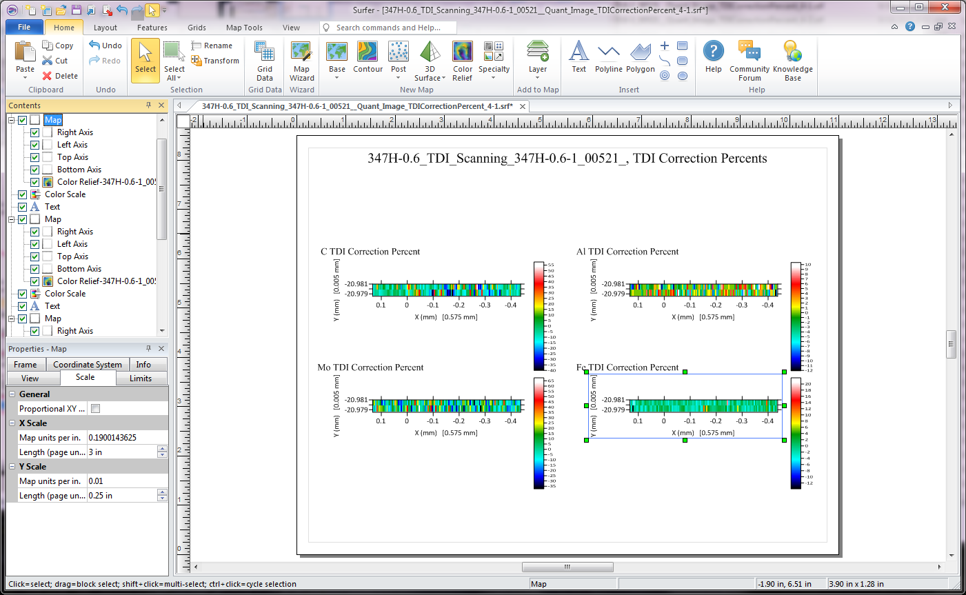
which reveals that the elements are all around a zero percent TDI correction with the exception of the carbon map, which is around minus 10% or so, with some variation at the single pixel level. This could be due to the observed presence of scattered sub micron carbide grains.
Finally the TDI corrected (and blank corrected ) maps for carbon and three other elements.
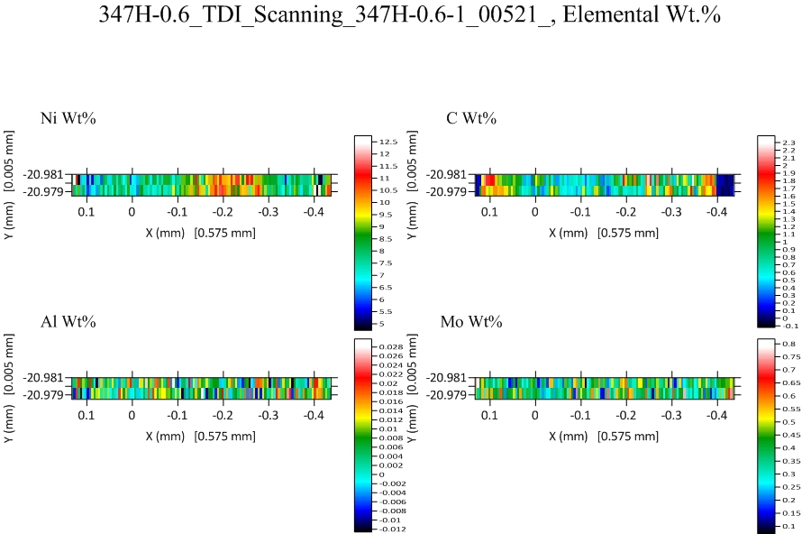
We can see that except for the edges of the sample, which consist of an oxidized zone, the average carbon concentration is around 0.5 wt% in the interior and also a slightly higher carbonized zone just at the oxide to metal transition on each side.


 We are a community of analysts, that cares about EPMA