Will the 'real' carbon coat density please stand up?

[JohnF]

Kerrick, who wrote the 'bible'? about carbon coating in American Mineralogist eons ago (American Mineralogist, Volume 58, pages 920-925, 1973, The Role of Carbon Film Thickness in Electron Microprobe Analysis) uses the density of the _coating_ (not the graphite rod) as 1.3 g/cc. However, PfE uses 2.1 g/cc.  Graphite is listed in the Google encyclopedia of knowledge) as: amorphous: 1.8–2.1 g/cm3; graphite: 2.267 g/cm3; diamond: 3.515 g/cm3.  Why is the Google value, maximum, of 2.1 being used? For all I know, Kerrick is wrong, and Mr. Google is correct, but what is the proof? Is there some reference where the carbon coat density has been directly (or indirectly) measured?

[Probeman]

Kerrick, who wrote the 'bible'? about carbon coating in American Mineralogist eons ago (American Mineralogist, Volume 58, pages 920-925, 1973, The Role of Carbon Film Thickness in Electron Microprobe Analysis) uses the density of the _coating_ (not the graphite rod) as 1.3 g/cc. However, PfE uses 2.1 g/cc.  Graphite is listed in the Google encyclopedia of knowledge) as: amorphous: 1.8–2.1 g/cm3; graphite: 2.267 g/cm3; diamond: 3.515 g/cm3.  Why is the Google value, maximum, of 2.1 being used? For all I know, Kerrick is wrong, and Mr. Google is correct, but what is the proof? Is there some reference where the carbon coat density has been directly (or indirectly) measured?

Hi John,
Interesting. I knew about Kerrick's work with regard to the electron energy loss calculation for the conductive coating, as that is what is used in CalcZAF and Probe for EPMA for correcting for differences in the coating between one's standards and unknowns.  But I did not notice his value for carbon density.  Interesting that it is so small.

As you say, it's variable, so enter whatever value you prefer.  That is why the field is editable!
john

[Mike Matthews]

Jurek et al, 1994 (Microchimica Acta) reports sputter coated C films as having ~ the same density as bulk graphite (2.25 g/cc) but vacuum evaporated films have significantly lower densities (1.3 - 2.0 g/cc), closer to but still generally lower than the bulk density value of amorphous C (1.8 - 2.1 g/cc).

Carbon's not the only material that can exhibit lower than bulk densities as thin films. I've just submitted a paper to MiMi which reports Al thin films with a density of ~2 g/cc compared to the bulk value of 2.7 g/cc.

[Ben Buse]

Stephen Reed in Electron Microprobe Analysis and Scanning Electron Microscopy in Geology quotes 2 g cm-3 citing Jurek et al 1994.

Ben

[JohnF]

Thank you Mike and Ben for your input. We are quite interested in this as we found that there was enough variation in the carbon coats on a sample vs the standard that the analytical totals were wacky, whereas the stoichiometry was perfect (plagioclase). Inputing different coat thickness values in PfE (from StrataGem k-ratios) saved the day. However, we noted that the thickness in StrataGem (which uses mass thickness) is a variable dependent upon density. So getting an accurate density would be rather useful.

[Probeman]

Thank you Mike and Ben for your input. We are quite interested in this as we found that there was enough variation in the carbon coats on a sample vs the standard that the analytical totals were wacky, whereas the stoichiometry was perfect (plagioclase). Inputing different coat thickness values in PfE (from StrataGem k-ratios) saved the day. However, we noted that the thickness in StrataGem (which uses mass thickness) is a variable dependent upon density. So getting an accurate density would be rather useful.

Hi John et al.,
I ran into this same carbon coat density question yesterday on a metallurgical sample I am running for another university.

Basically it's a Ti-Nb couple and quite interesting because, for this system the diffusitivities (is that the correct word?) are different by around 5 orders of magnitude, so Nb diffuses readily into Ti, but Ti will not diffuse into Nb. Really weird.

Anyway, the sample is uncoated, but the standards are coated with our usual 20 nm of carbon. So when I went to do the quant I got this output:

Un    4 Ti-Nb boundary, Results in Elemental Weight Percents
 
ELEM:       Ti      Nb       O
BGDS:      EXP     LIN     EXP
TIME:    40.00   40.00   40.00
BEAM:    30.01   30.01   30.01

ELEM:       Ti      Nb       O   SUM 
   210   -.009 101.534   1.173 102.698
   211   -.008 102.291   1.260 103.544
   212   -.001 101.548   1.245 102.792
   213   -.023 101.994   1.244 103.215
   214    .026 101.660   1.221 102.908
   215    .005 102.474   1.201 103.679
   216    .063 102.108   1.287 103.458
   217    .022 102.335   1.279 103.636
   218   -.006 101.594   1.209 102.797
   219    .043 101.464   1.317 102.824
   220    .003 101.527   1.241 102.771
   221   -.013 102.022   1.305 103.314
   222   -.001 101.583   1.252 102.833
   223    .030 101.848   1.171 103.049
   224    .019 101.799   1.305 103.123
   225    .035 102.506   1.309 103.849

This is using an 8 keV electron beam because they want the best spatial resolution they can get (we're doing another run tonight at 6 keV to try and further improve the spatial resolution and also to further reduce the SF effects).

Anyway, the above output clearly shows the need to specify the carbon coat for the standards and turn it off for the unknown.  For the unknown this is easily done from the Calculation Options dialog by unchecking the "Use Unknown Conductive Coating" checkbox.  For the standards one needs to use the Standard | Edit Standard Coating Parameters menu, but by default they are set to 200 nm of carbon at 2.1 gm/cm3.

Then one has to go into the Analytical | Analysis Options dialog and explicitly turn on the conductive coating correction by checking these two checkboxes:



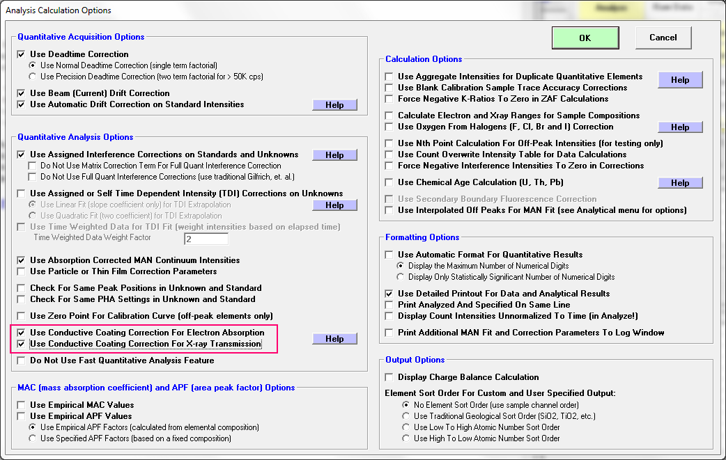
Once that is done we should be OK (or should we?), and we now obtain this analysis:

Un    4 Ti-Nb boundary, Results in Elemental Weight Percents
 
ELEM:       Ti      Nb       O
BGDS:      EXP     LIN     EXP
TIME:    40.00   40.00   40.00
BEAM:    30.01   30.01   30.01

ELEM:       Ti      Nb       O   SUM 
   210   -.008  95.301   1.024  96.316
   211   -.007  96.010   1.099  97.102
   212   -.001  95.313   1.086  96.398
   213   -.021  95.731   1.085  96.795
   214    .024  95.418   1.065  96.508
   215    .004  96.183   1.047  97.234
   216    .057  95.838   1.122  97.017
   217    .020  96.051   1.116  97.187
   218   -.005  95.357   1.054  96.406
   219    .040  95.232   1.149  96.421
   220    .003  95.293   1.083  96.379
   221   -.011  95.756   1.139  96.883
   222   -.001  95.345   1.092  96.436
   223    .028  95.596   1.021  96.645
   224    .017  95.547   1.138  96.703
   225    .032  96.210   1.142  97.384

So now our analysis is low!  Of course these coating effects are significantly amplified when running at low voltage (or low overvoltage), but we're pretty sure that the coating on our standards is close to 20 nm based on the color on polished brass as discussed here:

http://probesoftware.com/smf/index.php?topic=921.msg7063#msg7063

So then there's the density question and the consensus above seems to be that the evaporated deposited coatings are often less dense than their "accepted" values.  So I changed the carbon density from 2.1 to 1.4 and voila:

Un    4 Ti-Nb boundary, Results in Elemental Weight Percents
 
ELEM:       Ti      Nb       O
BGDS:      EXP     LIN     EXP
TIME:    40.00   40.00   40.00
BEAM:    30.01   30.01   30.01

ELEM:       Ti      Nb       O   SUM 
   210   -.008  97.376   1.072  98.439
   211   -.007  98.101   1.151  99.245
   212   -.001  97.389   1.137  98.524
   213   -.022  97.816   1.136  98.931
   214    .025  97.496   1.116  98.637
   215    .004  98.277   1.096  99.378
   216    .059  97.925   1.175  99.159
   217    .021  98.143   1.168  99.332
   218   -.005  97.433   1.104  98.532
   219    .041  97.307   1.203  98.550
   220    .003  97.368   1.134  98.505
   221   -.012  97.842   1.192  99.022
   222   -.001  97.422   1.143  98.564
   223    .029  97.677   1.069  98.775
   224    .018  97.629   1.192  98.838
   225    .033  98.306   1.195  99.534

You gotta admit, that's pretty impressive...

[JohnF]

Interesting, as we say, Mr. Donovan.

Back in the carbon film density saddle again.

With easy-to-access articles on the inter webs:
Characteristic Energy Losses of Electrons in Carbon, August 1960, Journal of Applied Physics, Vol 31, No 8 by Lewis Leder and J A Suddeth (NBS folks), their table 3 reports 1.35 density for evaporated carbon, citing the 1958 paper by W. Langbein, in Naturwissenschaften, 45, p. 510 entitled  (all in German) Elektroneninterferometrishce Messing des inneren Potentials von Kohlenstoff-Folien, which gives the density (experimental) as 1.35 +/- 0.03.

[Probeman]

Interesting, as we say, Mr. Donovan.

Back in the carbon film density saddle again.

With easy-to-access articles on the inter webs:
Characteristic Energy Losses of Electrons in Carbon, August 1960, Journal of Applied Physics, Vol 31, No 8 by Lewis Leder and J A Suddeth (NBS folks), their table 3 reports 1.35 density for evaporated carbon, citing the 1958 paper by W. Langbein, in Naturwissenschaften, 45, p. 510 entitled  (all in German) Elektroneninterferometrishce Messing des inneren Potentials von Kohlenstoff-Folien, which gives the density (experimental) as 1.35 +/- 0.03.

How cool is that!   Nice find!

I was just guessing the carbon density based on the totals, but if I specify a carbon density of 1.35 my totals are even closer to 100%:

Un    4 Ti-Nb boundary, Results in Elemental Weight Percents
 
ELEM:       Ti      Nb       O
BGDS:      EXP     LIN     EXP
TIME:    40.00   40.00   40.00
BEAM:    30.01   30.01   30.01

ELEM:       Ti      Nb       O   SUM 
   210   -.008  97.524   1.075  98.591
   211   -.007  98.250   1.155  99.398
   212   -.001  97.537   1.140  98.676
   213   -.022  97.965   1.140  99.083
   214    .025  97.645   1.119  98.789
   215    .004  98.427   1.100  99.531
   216    .059  98.075   1.179  99.312
   217    .021  98.293   1.172  99.485
   218   -.005  97.582   1.107  98.684
   219    .041  97.455   1.207  98.703
   220    .003  97.516   1.137  98.657
   221   -.012  97.991   1.196  99.175
   222   -.001  97.570   1.147  98.716
   223    .029  97.826   1.073  98.927
   224    .018  97.777   1.196  98.991
   225    .033  98.456   1.199  99.688

You know what this means?  It means we should all change our default carbon density in our probewin.ini file to 1.35!

This keyword is found in the [standards] section of the probewin.ini file (usually C:\ProgramData\Probe Software\Probe for EPMA) as seen here:

StandardCoatingFlag=1       ; 0 = not coated, 1 = coated
StandardCoatingElement=6   ; assume carbon
StandardCoatingDensity=1.35
StandardCoatingThickness=200   ; in angstroms

I'm going to have to change all the default coating density parameters in my example config files!

[Mike Matthews]

Just to throw another spanner in the works: I'm sure we've all seen ring-shaped carbon contamination formed around a static beam spot, but did you know the centre of the ring can exhibit net carbon erosion? It doesn't even need particularly aggressive analysis conditions: I've measured 1.1nm loss over 60s with a 25nA FEG beam at 5kV. When the starting thickness is 5nm this represents a serious proportional loss. PfE's TDI analysis mode copes admirably well with correcting the changing emitted intensities.

[Probeman]

Just to throw another spanner in the works: I'm sure we've all seen ring-shaped carbon contamination formed around a static beam spot, but did you know the centre of the ring can exhibit net carbon erosion? It doesn't even need particularly aggressive analysis conditions: I've measured 1.1nm loss over 60s with a 25nA FEG beam at 5kV. When the starting thickness is 5nm this represents a serious proportional loss. PfE's TDI analysis mode copes admirably well with correcting the changing emitted intensities.

Hi Mike,
I think I have observed this effect also, but not really knowing what I was seeing:

http://probesoftware.com/smf/index.php?topic=48.msg160#msg160

See the attachment in the post linked above, and notice the slight decrease in carbon intensity for the first few points (at least until the electron beam starts encroaching on the deposited carbon "ring").
john

[jon_wade]

Off topic slightly, but carbon related all the same - anyone know if peaksight takes any account of carbon coatings?  I am not sure - my doubts are raised by the fact  you can't specify its presence or absence for an unknown.....