Author Topic: Nasty Boundary Fluorescence Analytical Situations  (Read 58056 times)

jon_wade

  • Professor
  • ****
  • Posts: 82
Re: Nasty Boundary Fluorescence Analytical Situations
« Reply #45 on: December 04, 2017, 02:16:08 PM »
John - nice poster.  You  modelled the melt inclusion with FANAL, but the region of interest is pretty small (0.25 um to 4um).  The effects of direct interaction would really exacerbate the effect and have a big effect on the interpretation of this data when stripped out.  You should point this out to the diffusion crowd.

Probeman

  • Emeritus
  • *****
  • Posts: 2856
  • Never sleeps...
    • John Donovan
Re: Nasty Boundary Fluorescence Analytical Situations
« Reply #46 on: December 04, 2017, 02:35:00 PM »
John - nice poster.  You  modelled the melt inclusion with FANAL, but the region of interest is pretty small (0.25 um to 4um).  The effects of direct interaction would really exacerbate the effect and have a big effect on the interpretation of this data when stripped out.  You should point this out to the diffusion crowd.

Hi Jon,
We just submitted a paper to Chemical Geology with Anastassia Borisova (Grenoble) as first author, and Xavier, Paul Asimov (Cal Tech) and myself and others on this very topic!

I sort of instigated this effort after I went to AGU last year, and to my shock around a third of the diffusion profiles I saw in presentations were mostly (if not completely) secondary fluorescence artifacts!
john
The only stupid question is the one not asked!

Probeman

  • Emeritus
  • *****
  • Posts: 2856
  • Never sleeps...
    • John Donovan
Re: Nasty Boundary Fluorescence Analytical Situations
« Reply #47 on: May 22, 2018, 10:57:27 AM »
I'm happy to say that our paper on secondary fluorescence issues in geological samples has been published.  A free link (for 50 days I think) is here:

https://www.sciencedirect.com/science/article/pii/S0009254118302304

Also I've attached a pdf of the paper below (please login to see attachments).
john
The only stupid question is the one not asked!

jon_wade

  • Professor
  • ****
  • Posts: 82
Re: Nasty Boundary Fluorescence Analytical Situations
« Reply #48 on: May 23, 2018, 02:52:46 PM »
no idea who reviewed it.....

Probeman

  • Emeritus
  • *****
  • Posts: 2856
  • Never sleeps...
    • John Donovan
Re: Nasty Boundary Fluorescence Analytical Situations
« Reply #49 on: May 23, 2018, 03:09:00 PM »
no idea who reviewed it.....

Ha!

But we certainly appreciated the reviewer's very helpful suggestions nonetheless...     :)
« Last Edit: May 23, 2018, 03:17:37 PM by Probeman »
The only stupid question is the one not asked!

Probeman

  • Emeritus
  • *****
  • Posts: 2856
  • Never sleeps...
    • John Donovan
Re: Nasty Boundary Fluorescence Analytical Situations
« Reply #50 on: October 01, 2018, 04:27:50 PM »
After posting about heterogeneous interaction volumes and secondary fluorescence at boundaries I decided to take a more real world example than the simple Fe-Ni boundary. So here is a FeNi alloy adjacent to pure Ni:


A negative drop of 1.5% absolute in the Fe concentration and still significant at 10 um from the boundary!  The physics gods have their revenge on us!  The world is complicated to model!

After I posted the above I realized that a more "real world" example would be FeNi alloy adjacent to epoxy, but as expected, it's pretty much the same effect:


Remember: the effects you are seeing here are *NOT* due to electrons "leaking" into the Ni or epoxy. The calculation assumes that all electrons come to rest in the "beam incident" material.
« Last Edit: October 01, 2018, 04:36:18 PM by Probeman »
The only stupid question is the one not asked!

Probeman

  • Emeritus
  • *****
  • Posts: 2856
  • Never sleeps...
    • John Donovan
Re: Nasty Boundary Fluorescence Analytical Situations
« Reply #51 on: October 02, 2018, 01:23:36 PM »
And just in case anyone else is wondering, yes, these "self" secondary fluorescence effects at boundaries can also occur for silicates!

Here is an example of iron in fayalite measured adjacent to anorthite. The iron in the olivine is being self fluoresced by the continuum radiation produced by the electron beam, but since there is no iron in the anorthite (or at least not much), as the analysis position approaches the boundary, the Fe signal decreases because there is no Fe in the anorthite that can be fluoresced by the continuum radiation produced in the beam incident material.


This decrease is significant even 10 to 15 um away from the boundary. Again, not because of electron leakage into the boundary material, but because, you know, physics.  :)
« Last Edit: October 02, 2018, 01:26:54 PM by Probeman »
The only stupid question is the one not asked!

jrminter

  • Professor
  • ****
  • Posts: 72
Re: Nasty Boundary Fluorescence Analytical Situations
« Reply #52 on: October 04, 2018, 10:23:40 AM »
That is a really nice example. I wanted to see how close one needed to get to the boundary to get a significant C X-ray from the Epoxy. DTSA-II has a nice python function (interface() in the mcSimulate3.py file in the lib directory) to permit one to analyze such a system where one places a secondary material (Epoxy) at a specified distance from the primary material (NBS NiFe). CalcZAF has these materials in the database, so it was easy for me to create the DTSA-II materials and put them into the DTSA-II database and I wrote a python script to do the simulation. I am attaching two images: 1) overlay of spectra with the boundary 0.25, 0.5, and 2.0 microns from the C and 2) a montage of the three C emission images. My apologies to those who have R-G colorblindness. DTSA uses R & G as default colors as part of the first three spectra.

Probeman

  • Emeritus
  • *****
  • Posts: 2856
  • Never sleeps...
    • John Donovan
Re: Nasty Boundary Fluorescence Analytical Situations
« Reply #53 on: October 06, 2018, 09:50:42 AM »
Here's the same C Ka in Fe2SiO4 calculation in Standard using the Penfluor/Fanal GUI:


The magnitude of the SF effect is highly dependent on how penetrating the emitted x-ray is, and for carbon it's not much. By comparison, for a high energy x-ray such as Zn Ka, one can obtain a 100 PPM signal in a Al or Mg matrix up to 500 um away from the boundary!


Here is the same geometry but calculated out to 500 um from the boundary and plotted on a log scale:


These calculations suggest to us that if we want to avoid SF boundary effects, then we should try to utilize the lowest energy emission line possible. So switching this Al/Zn boundary to the Zn La line, we obtain this:


Which is more similar to the C Ka emission plot above.
The only stupid question is the one not asked!

Probeman

  • Emeritus
  • *****
  • Posts: 2856
  • Never sleeps...
    • John Donovan
Re: Nasty Boundary Fluorescence Analytical Situations
« Reply #54 on: October 08, 2018, 12:42:20 PM »
I realized today that the C Ka adjacent to epoxy calculation I did was for Fe2SiO4, while John Minter's calculation was for a NiFe alloy.  So I recalulated the NBS NiFe alloy down to 200 eV to capture the carbon intensity and the results are seen here:


Note the high absorption of C ka in the difference between the concentration at 30 PPM and the k-ratio at 5 PPM.

If anyone would like to play with these low keV calculations I've attached a ZIP file below with a number of PAR files calculated to below 1 keV. Just unzip these folders to your Penepma12\Penfluor folder and you can load them into the Standard app for modeling.  Remember you need to login to see attachments.
john
The only stupid question is the one not asked!

macosta

  • Graduate
  • **
  • Posts: 9
Re: Nasty Boundary Fluorescence Analytical Situations
« Reply #55 on: March 07, 2019, 02:05:05 PM »
SF effect of non-contiguous TiO2 phase when measuring Ti in quartz?

Hello all,

I am measuring Ti in individual quartz grains (less than 20 micron long diameter). Problematically, there are small (approximately <5 micron long diameter) TiO2 particles interspersed densely throughout my sample. I did most of my analyses in the centers of crystals that were as far away from the TiO2 phase as possible, ~40 micron away from the nearest particle in most cases. See image below.

I am unfamiliar with modeling complex geometries in Penepma and am hoping that someone has encountered a similar issue and will be able to help. The problem is that the grain of interest is separated from the contaminant crystal in multiple directions by several grain boundaries as well as epoxy. Any help is greatly appreciated,

-Marisa
Marisa D. Acosta

Probeman

  • Emeritus
  • *****
  • Posts: 2856
  • Never sleeps...
    • John Donovan
Re: Nasty Boundary Fluorescence Analytical Situations
« Reply #56 on: March 08, 2019, 05:28:33 PM »
SF effect of non-contiguous TiO2 phase when measuring Ti in quartz?

Hello all,

I am measuring Ti in individual quartz grains (less than 20 micron long diameter). Problematically, there are small (approximately <5 micron long diameter) TiO2 particles interspersed densely throughout my sample. I did most of my analyses in the centers of crystals that were as far away from the TiO2 phase as possible, ~40 micron away from the nearest particle in most cases. See image below.

I am unfamiliar with modeling complex geometries in Penepma and am hoping that someone has encountered a similar issue and will be able to help. The problem is that the grain of interest is separated from the contaminant crystal in multiple directions by several grain boundaries as well as epoxy. Any help is greatly appreciated,

-Marisa

Hi Marisa,
This sort of thing can get complicated real fast.  I try to approach complicated things by first looking at worst case but simplified models. So we already know, using the quick secondary fluorescence GUI for Penfluor/Fanal in Standard (CalcZAF), that if our TiO2 is 40 um away (and I'll assume you're running 15 keV, but maybe not, though it won't be a big effect if you're at 20 keV), the apparent signal from TiO2 is about 0.05 wt% Ti SF effect for an infinite boundary between SiO2 and TiO2.  Or 500 PPM. This SiO2/TiO2 SF calculation is described step by step here:

https://probesoftware.com/smf/index.php?topic=58.msg214#msg214

But that doesn't apply to your situation of a 5 um (or less) TiO2 inclusion. So we need to pull out the "big gun" and run the Penepma model using the geometric model for an inclusion in a matrix. Instructions for running Penepma are here:

https://probesoftware.com/smf/index.php?topic=322.0

But the discussion on modeling inclusions using Penepma is here:

https://probesoftware.com/smf/index.php?topic=59.0

Probably should be updated...

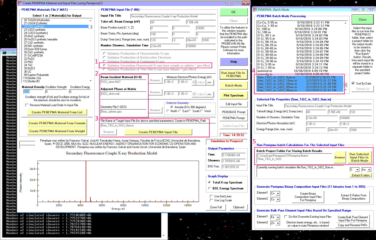
So anyway, our next simple but a little more accurate model would be to use Penepma for a 5 um particle inclusion. In this screen shot I created input files for a 5 um TiO2 particle 0, 10, 20, 40 and 80 microns away from the beam position. The 0 um beam position will be in the center of the 5 um TiO2 particle and we can use that as a pseudo standard for the k-ratio (I just realized that I should have added 2.5 microns to all the non-zero distances due to the radius of the 5 um inclusion. Oh well).

Anyway, here is the screen shot, which also shows the basic steps to create the input files and run them from the Penepma batch window:


So you should feel free to play around with these Penfluor/Fanal and Penepma GUI interfaces, especially if your samples were run at 20 keV and (oops!), I see from your BSE image that you did. So yes, you should re-do what I'm doing but at 20 keV. But on Monday we can look at the 15 keV models and see what we get.

The point will be that instead of 500 PPM Ti SF effect, we'll get something much smaller. Then the next thing to consider is the fact that you've also got some epoxy in between your SiO2 and your 5 um TiO2 particle.  So what will that do?

Well since we know that no characteristic emission lines will be produced from SiO2 that are capable of fluorescing the Ti K edge, we need to only think about continuum emission from the SiO2, and again, only those continuum x-rays that have enough energy to fluoresce the Ti Ka edge in our 5 um TiO2 particle.

To model this in Penepma, will require the use of three materials in our geometric model. Jon Wade and I did create some "trilayer" .geo files but these are intended for a substrate with two thin films deposited on it, so there would some work needed to create a .geo file specifically for your SF situation with SiO2, TiO2 and epoxy.

In the meantime we can imagine what might happen if there was some intervening epoxy between our SiO2 and our TiO2. The continuum x-rays will be produced at the beam incident spot and will travel (roughly) in a spherical direction and until they reach our 5 um TiO2 particle. What will the intervening epoxy do to these high energy continuum x-rays (between 5 and 15 or 20 keV)?

Specifically will these continuum x-rays will tend to be more absorbed by epoxy or less absorbed by epoxy, than SiO2? Nothing like running a physics model I say, so I used Mn Ka traversing 40 um of both SiO2 matrix and epoxy, to see what happens to x-rays that are enough to excite the Ti K edge. Because the Mn Ka is 5.89 keV and the Ti K edge is 4.96 keV so Mn Ka will be a "stand-in" for our high energy continuum x-rays until we do a proper modeling in Penepma with three materials in the proper geometry.

So using the Model Electron and X-Ray Ranges window in CalcZAF, I looked at 40 um of SiO2 for Mn Ka:

Si-O2 = Si1O2 =  60.086g/mol, Si 46.74%  O 53.26%
15 keV, 2.7 grams/cm^3
Electron range radius = 2.449919 um
Mn ka, at 15 keV, (6.539 keV edge energy)
X-ray production range radius = 1.837592 um
mn ka absorbed by si =  145.0962
mn ka absorbed by o  =  28.13147
Mn ka, x-ray transmission fraction through thickness 40 um (average u/p = 82.8043) = 0.4088993

So about 40% of the Mn Ka x-rays are transmitted through 40 um of SiO2.

And here for Mn Ka in epoxy:

15 keV, 1.16 grams/cm^3
Electron range radius = 5.316666 um
Mn ka, at 15 keV, (6.539 keV edge energy)
X-ray production range radius = 3.987831 um
mn ka absorbed by c  =  10.91245
mn ka absorbed by h  =  .01601
mn ka absorbed by o  =  28.13147
mn ka absorbed by cl =  240.9663
Mn ka, x-ray transmission fraction through thickness 40 um (average u/p = 14.06128) = 0.9368385

So about 93% of these Mn Ka x-rays (acting as a "stand-in" for our high energy continuum x-ray that would tend to fluoresce the Ti K edge), will get transmitted through epoxy.

So Mn Ka is a lot less absorbed by epoxy than by SiO2, so whatever SF effect we see in our Penepma modeling, it will be somewhat larger when we run a Penepma model with intervening epoxy.  So your question turns out to be very important!  We would be underestimating the SF effect if there is some epoxy in between our SiO2 and our TiO2 inclusion!

Now on the other hand, depending on the beam position and TiO2 orientation to the WDS spectrometer, there may also be Bragg defocus effects which will tend to *reduce* the SF effect:

https://www.cambridge.org/core/journals/microscopy-and-microanalysis/article/secondary-fluorescence-in-wds-the-role-of-spectrometer-positioning/94F6F5D3992B37BFBB8B4116BB4605D3

Told you it gets complicated!   :D   Let's see what we get on Monday and we can take it from there.

Unless someone has already run these models and can share them with us?
« Last Edit: March 08, 2019, 07:58:16 PM by Probeman »
The only stupid question is the one not asked!

Probeman

  • Emeritus
  • *****
  • Posts: 2856
  • Never sleeps...
    • John Donovan
Re: Nasty Boundary Fluorescence Analytical Situations
« Reply #57 on: March 11, 2019, 04:07:24 PM »
I'm waiting for the 40 um distance from a 5 um TiO2 inclusion Penepma run to finish and I'll post those results tomorrow, but I could really use some help from someone with experience in Penepma .geo files to create a .geo file for 3 materials for us with a geometry shown in the attachment below.

The idea being that we could run it twice, once with epoxy as the matrix and a second time with SiO2 as the matrix.

Thanks!
The only stupid question is the one not asked!

Probeman

  • Emeritus
  • *****
  • Posts: 2856
  • Never sleeps...
    • John Donovan
Re: Nasty Boundary Fluorescence Analytical Situations
« Reply #58 on: March 12, 2019, 11:29:52 AM »
OK, I've got some preliminary results at 15 keV for a 5 um TiO2 particle in an SiO2 matrix:

"Ti ka in Sample"    "Distance or Radius (um)"    "Std.Tot.Int."    "Unk.Tot.Int."    "Unk.Tot.Int.Var."    "K-ratio"    "K-ratio Var."
"5um_TiO2_in_SiO2_10um"          2.5                4.97e-05           2.29e-09           5.90e-10            .000046     .000012
"5um_TiO2_in_SiO2_20um"          2.5                4.97e-05           5.06e-10           2.87e-10            .000010     .000006
"5um_TiO2_in_SiO2_40um"          2.5                4.97e-05           1.21e-10           1.37e-10            .000002     .000003

These k-ratios where calculated using the Extract K-Ratios button in the Standard app, from the Penepma Batch Mode window as described here:

https://probesoftware.com/smf/index.php?topic=202.msg1506#msg1506

For the standard intensity I simply utilized the 0 um distance TiO2 particle model, which isn't exactly correct, but for a trace element, it works just fine.

Note that the "Distance or Radius (um) only refers to the radius of the inclusion which was 5 um in diameter.  The actual distances (because I forgot to add the inclusion radius to my beam location distance) are 7.5, 17.5 and 37.5 um.

So converting the k-ratios to % k-ratio and applying a matrix correction of ~1.2 (TiO2 std k-factor = 0.5546) for Ti Ka in SiO2 we get the following results:

                       Dist from inclu      k-ratio        % k-ratio         wt% matrix corrected
"5um_TiO2_in_SiO2_10um"    7.5                .000046          .0046         .00300           (30 PPM)
"5um_TiO2_in_SiO2_20um"    17.5               .000010          .0010         .00066          (6.6 PPM)
"5um_TiO2_in_SiO2_40um"    37.5               .000002          .0002         .00013          (1.3 PPM)

Therefore we're seeing only about 1-2 PPM SF effect from a 5 um TiO2 particle 40 (37.5) um away from our beam spot in SiO2.  I have to admit, it surprises me a bit that at 7.5 um from a 5 um particle and we're only getting 30 PPM of SF effect.   Can anyone confirm these calculations?

Next question is how much SF effect will there be when we replace some of that 40 um of SiO2 with epoxy?

Also, does anyone have a .geo file for the geometry for three materials as described in the attachment in the above post (please login to see attachments)?
« Last Edit: March 12, 2019, 05:50:54 PM by Probeman »
The only stupid question is the one not asked!

Probeman

  • Emeritus
  • *****
  • Posts: 2856
  • Never sleeps...
    • John Donovan
Re: Nasty Boundary Fluorescence Analytical Situations
« Reply #59 on: March 13, 2019, 10:04:07 AM »
I am reminded of a talk I heard here a few weeks ago from a highly regarded Professor at a California school which shall remain nameless.  There was a particular slide claiming to see differential diffusion profiles towards a grain boundary.  Some quick modeling after the talk showed that it could all be explained by secondary fluorescence.  I know the three Jo/h/n's (Wade, Donovan, and Fournelle) are adamant about trying to educate the public.  What can we do to actually make this point sink in?

Anyways:  There are essentially two solutions to this problem as Ben mentioned

1) Acquire the data normally and run it through PENEPMA, modeling the influence of secondary fluorescence.  Then removing the influence of secondary fluorescence on each data point during the transect towards the grain boundary.  A bit time consuming right now, but I wonder if PfEPMA wouldn't be able to do that quite easily now that is has the modeling built in.....

2) Alternatively use the non-traditional lines J.D. mentioned and use low accelerating potential (<8 keV).  The influence of secondary fluorescence goes away for most elements in this case.  You could also use the normal L lines if all you are after is the diffusion profile, and not absolute concentrations.

Hi Phil,
I realize this is a two year old post, but it's worth mentioning again that now there is a geology paper on these SF effects:

https://www.sciencedirect.com/science/article/pii/S0009254118302304

john
The only stupid question is the one not asked!