Author Topic: Compound or Specified Area Peak Factors (APFs)  (Read 5847 times)

Probeman

  • Emeritus
  • *****
  • Posts: 2856
  • Never sleeps...
    • John Donovan
Compound or Specified Area Peak Factors (APFs)
« on: June 24, 2015, 01:21:09 PM »
Ok, here's a short tutorial on obtaining area peak factors (APFs) using boron as an example.  Be aware however, that for low intensity boron peaks, e.g., boro-silicates, the background fitting is quite crucial for best accuracy.

So let's say we wanted to analyze boron nitride using boron metal as a standard. Assuming you've properly polished and coated your materials (also crucial for low energy emission lines such as oxygen, nitrogem carbon, boron, etc) and properly set up your peaking and PHA (here we peaked on our primary standard, boron metal), we then perform a high precision wavescan on both boron metal and boron nitride.  In this particular run I was analyzing magnesium boride unknowns, but since boron nitride peak shapes have been measured by Bastin, we can compare our results to his measurements.


So here is a scan on boron metal:


and by clicking the Model background button we can see the background fit and by clicking the Integrate button as seen here, we get our peak and integrated intensities:


Since boron metal is our primary standard, we make a note of the Peak/Integ (St) value of 7.25. Now we plot our boron nitride sample as seen here:


Note that there is a significant peak shift in the peak of boron nitride relative to boron metal. Not surprising, but this matter for your analytical setup in that it might be better to analyze each material at it's own peak position to avoid peak *shift* effects and just correct for peak *shape* effects.  We will visit this issue later.

Now we model the peak shape by again clicking the Model backgrounds button as seen here:


and this time we make a note of the Integ/peak (Un) value of 0.167 because in this particular example, boron nitride is our "unknown".  Now multiplying these two numbers, we obtain an APF of 1.21 which seems a little high, especially when compared to Bastin's boron in boron nitride value of 1.20. 

Ok, now you thinking "hey these are pretty close actually", but the problem is Bastin used a Pb stearate crystal which has a much higher spectral resolution compared to the PC25 multi-layer crystal I used. So really the APF for the PC25 crystal should be much closer to 1.0, so why is that?

Well it's because we have included the peak *shift* effect in our APF calculation and instead Bastin re-peaked each scan on both the boron metal and the boron nitride materials to focus on the peak shape effects only.

So, what if we re-peak our boron nitride scan for the peak intensity?   But there is no need to re-run the scan, let's just re-fit the peak intensity as seen here:


How did we do that, from the Model backgrounds dialog we merely clicked the Maxima peak fit option before we clicked the Integrate button as seen here:


So now we obtain a Integ/Peak (Un) value of 0.143 and multiplying that with our original boron meta Peak/Integ (St) value of 7.25 we now get an APF of 1.036, which is much closer to what we would expect for peak *shape* effects only on a low resolution LDE crystal.

I'd be pleased to answer any questions you may have. I've also attached a write up on my magnesium boride efforts (remember you have to be logged in to see attachments!).
« Last Edit: July 01, 2015, 04:55:49 PM by John Donovan »
The only stupid question is the one not asked!

John Donovan

  • Administrator
  • Emeritus
  • *****
  • Posts: 3304
  • Other duties as assigned...
    • Probe Software
Re: Compound or Specified Area Peak Factors (APFs)
« Reply #1 on: July 01, 2015, 05:20:55 PM »
I've recently modified the peak integration code in the Plot! window Model Backgrounds dialog to only integrate the peak area between the high and low off-peak background positions.

This is consistent with the integrated intensity scan acquisition option seen here in the Elements/Cations dialog:


By the way, before I go on further with the APFs, this integrated intensity acquisition option in PFE is quite nice because at low intensities the scan step size is larger, and as the peak intensity increases, the step size decreases automatically, to allow more time to be spent on the peak itself as opposed to the background intensities.

To see the acquired integrated intensity acquisitions just click the Run | Display Integrated Intensities menu and you will see this:


If we now zoom in on the side of the peak we can see this "variable" integrated intensity acquisition step size as seen here:


Anywho, back to the area peak factor (APF) method, which allows us to characterize the peak shape effects prior to acquisition for improved light element quant without having to spend all that time "crawling" over the peak!

So, here is an example of a linear fit to a wavescan on Al2O3 with O ka:


The Model background dialog looked like this:


Note the not quite perfect fit to the background and to get the most accurate integrated area under the peak we'll want to fit better. Now here is the same data but the background is fit to an exponential fit:


and here is what the Model backgrounds dialog looked like:


Note the smaller fitting problem with the exponential fit.  This modified code will produce improved integrated area intensity calculations for the creation of your own specified (or binary compound) area peak factors.
John J. Donovan, Pres. 
(541) 343-3400

"Not Absolutely Certain, Yet Reliable"

John Donovan

  • Administrator
  • Emeritus
  • *****
  • Posts: 3304
  • Other duties as assigned...
    • Probe Software
Re: Compound or Specified Area Peak Factors (APFs)
« Reply #2 on: July 01, 2015, 10:57:49 PM »
To sum up...

Once we have the peak and integrated intensities for our standard material and our secondary std or unknown, we multiply the peak:integrated intensity ratios as described here in the reference manual:

http://probesoftware.com/download/PROBEWIN.pdf#page=321

and obtain the desired light element area peak factor (APF). This resulting APF factor could be a single use "specified" APF for use in the Elements/Cations dialog as seen here:


where the APF was calculated by utilzing a "Standard" wavescan on the standard for the emitting element and a "Unknown" wavescan on the actual unknown material of interest.

Or these peak to integrated intensity ratios could be utilized for calculating compound binary APFs where the "Standard" wavescan is again on the primary standard for the light element emission line and the "Unknown" wavescan is on a secondary (binary composition) standard containing the light element emitting line of interest and one of the matrix elements bonded to the emitting element as shown in this dialog accessed from the Run | Empirical APFs menu as seen here:


The Model backgrounds dialog provides both ratios for your convenience. The benefit of the binary compound APFs is that they can be applied, to arbitrary compositions iteratively in the matrix correction, weighted based on the concentrations of each absorber (bonding) element to the light element emission line of interest as seen here:


The only "catch" for using binary compound APfs is that you must edit the EmpAPF.dat file as described in the manual so the user can select the necessary "empirical" APFs from the app for the situation at hand.

Why? Because the specific binary APFs selected will depend on the actual spectrometer crystal utilized for the wavescans and analysis (they must be the same and for JEOL users the spectrometer focal circle should also be the same), the compound bonding valance and lastly the crystal coordination for ultimate accuracy.  The following is a list of measured APFs from Bastin, Pouchou and myself that are distributed with CalcZAF and Probe for EPMA:

  "b"     "ka"    "c"        1.02         "B4C/B/STE"
  "b"     "ka"    "n"        1.2          "BN/B/STE"
  "b"     "ka"    "n"        1.214        "BN/B/PC25/147.6 Donovan"
  "b"     "ka"    "mg"       1.017        "MgB4/B/PC25/147.6 Donovan"
  "b"     "ka"    "mg"       0.937        "MgB2/B/PC25/147.6 Donovan"
  "b"     "ka"    "al"       1.12         "AlB2/B/STE"
  "b"     "ka"    "al"       1.01         "AlB12/B/STE"
  "b"     "ka"    "si"       1            "SiB3/B/STE"
  "b"     "ka"    "si"       .92          "SiB6/B/STE"
  "b"     "ka"    "ti"       .75          "TiB/B/STE"
  "b"     "ka"    "ti"       .88          "TiB2/B/STE"
  "b"     "ka"    "v"        1.           "VB2/B/STE"
  "b"     "ka"    "cr"       .9           "CrB/B/STE"
  "b"     "ka"    "cr"       1.1          "CrB2/B/STE"
  "b"     "ka"    "fe"       1.1          "FeB/B/STE"
  "b"     "ka"    "fe"       1.25         "Fe2B/B/STE"
  "b"     "ka"    "co"       1.2          "CoB/B/STE"
  "b"     "ka"    "co"       1.02         "Co2B/B/STE"
  "b"     "ka"    "ni"       1.2          "NiB/B/STE"
  "b"     "ka"    "ni"       1.06         "Ni2B/B/STE"
  "b"     "ka"    "ni"       .98          "Ni3B/B/STE"
  "b"     "ka"    "zr"       .8           "ZrB2/B/STE"
  "b"     "ka"    "nb"       .8           "NbB/B/STE"
  "b"     "ka"    "nb"       .9           "NbB2/B/STE"
  "b"     "ka"    "mo"       .94          "MoB/B/STE"
  "b"     "ka"    "la"       .9           "LaB6/B/STE"
  "b"     "ka"    "ta"       .88          "TaB/B/STE"
  "b"     "ka"    "ta"       1.1          "TaB2/B/STE"
  "b"     "ka"    "w"       .98          "WB/B/STE"
  "b"     "ka"    "u"       1.04         "UB4/B/STE"
  "c"     "ka"    "b"       1.16         "B4C/TiC/WSi/59.8"
  "c"     "ka"    "mg"      1.2          "MgB2C2/C/WSi/59.8"
  "c"     "ka"    "si"      1.07         "SiC/TiC/WSi/59.8"
  "c"     "ka"    "ti"      1.000000         "TiC/TiC/WSi/59.8"
  "c"     "ka"    "v"       1.005760         "V2C/TiC/WSi/59.8"
  "c"     "ka"    "v"       1.005760         "VC/TiC/WSi/59.8"
  "c"     "ka"    "cr"      0.921659         "Cr7C3/TiC/STE"
  "c"     "ka"    "cr"      0.95622          "Cr3C2/TiC/STE"
  "c"     "ka"    "cr"      0.921659         "Cr23C6/TiC/STE"
  "c"     "ka"    "zr"      1.013825         "ZrC/TiC/WSi/59.8"
  "c"     "ka"    "nb"      0.91013          "NbC/TiC/STE"
  "c"     "ka"    "mo"      0.94470          "Mo2C/TiC/STE"
  "c"     "ka"    "hf"      0.95622          "HfC/TiC/STE"
  "c"     "ka"    "ta"      1.105991         "TaC/TiC/STE"
  "c"     "ka"    "w"       1.117512         "WC/TiC/STE"
  "c"     "ka"    "w"       1.175115         "W2C/TiC/STE"
  "n"     "ka"    "si"      1.103          "Si3N4/AlN/WSi/59.8"
  "n"     "ka"    "ti"       .997          "TiN/AlN/WSi/59.8"
  "n"     "ka"    "v"       1.0226         "VN/AlN/WSi/59.8"
  "n"     "ka"    "cr"      1.018          "Cr2N/AlN/WSi/59.8"
  "n"     "ka"    "fe"      1.012          "Fe2N/AlN/WSi/59.8"
  "n"     "ka"    "zr"       .9952         "ZrN/AlN/WSi/59.8"
  "n"     "ka"    "hf"      1.002          "HfN/AlN/WSi/59.8"
  "o"     "ka"    "b"       1.0628        "B6O/Fe2O3/WSi/59.8"
  "o"     "ka"    "na"       1.0          "----/Fe2O3/WSi/59.8"
  "o"     "ka"    "mg"       1.0000       "MgO/Fe2O3/WSi/59.8"
  "o"     "ka"    "al"       1.0213       "Al2O3/Fe2O3/WSi/59.8, Bastin"
  "o"     "ka"    "al"       1.0285       "Al2O3/MgO/WSi/59.8, Donovan"
  "o"     "ka"    "si"       1.0444       "SiO2/Fe2O3/WSi/59.8, Bastin"
  "o"     "ka"    "si"       1.070        "SiO2/MgO/WSi/59.8, Donovan"
  "o"     "ka"    "p"        1.05         "----/Fe2O3/WSi/59.8"
  "o"     "ka"    "s"        1.2          "----/Fe2O3/WSi/59.8"
  "o"     "ka"    "k"        1.0          "----/Fe2O3/WSi/59.8"
  "o"     "ka"    "ca"       0.97         "----/Fe2O3/WSi/59.8"
  "o"     "ka"    "ti"       .9796        "TiO2/Fe2O3/WSi/59.8"
  "o"     "ka"    "cr"       .993         "Cr2O3/Fe2O3/WSi/59.8, Bastin"
  "o"     "ka"    "cr"       1.1         "Cr2O3/MgO/WSi/59.8, Donovan"
  "o"     "ka"    "mn"       1.0121       "MnO/Fe2O3/WSi/59.8"
  "o"     "ka"    "fe"       .9962        "Fe3O4/Fe2O3/WSi/59.8"
  "o"     "ka"    "co"       1.0133       "CoO/Fe2O3/WSi/59.8"
  "o"     "ka"    "ni"       1.0153       "NiO/Fe2O3/WSi/59.8"
  "o"     "ka"    "cu"       .9946        "Cu2O/Fe2O3/WSi/59.8"
  "o"     "ka"    "cu"       .9943        "CuO/Fe2O3/WSi/59.8"
  "o"     "ka"    "zn"       .9837        "ZnO/Fe2O3/WSi/59.8"
  "o"     "ka"    "ga"       1            "Ga2O3/Fe2O3/WSi/59.8"
  "o"     "ka"    "zr"       .9823        "ZrO2/Fe2O3/WSi/59.8"
  "o"     "ka"    "nb"       .9840        "Nb2O5/Fe2O3/WSi/59.8"
  "o"     "ka"    "mo"       .9940        "MoO3/Fe2O3/WSi/59.8"
  "o"     "ka"    "ru"       1.0109        "RuO2/Fe2O3/WSi/59.8"
  "o"     "ka"    "sn"       .9737        "SnO2/Fe2O3/WSi/59.8"
  "o"     "ka"    "tb"       1.2          "----/Fe2O3/WSi/59.8"
  "o"     "ka"    "ta"       1.0102        "Ta2O5/Fe2O3/WSi/59.8"
  "o"     "ka"    "w"       1.0099        "WO3/Fe2O3/WSi/59.8"
  "o"     "ka"    "pb"       0.9651        "PbO/Fe2O3/WSi/59.8"
  "o"     "ka"    "bi"       0.9754        "Bi2O3/Fe2O3/WSi/59.8"
  "al"    "ka"    "o"        1.06           "Al2O3/Al/TAP/25.745"
  "si"    "ka"    "o"        1.04           "SiO2/Si/TAP/25.745"
  "si"    "ka"    "o"        1.21           "SiO2/Si/PET/8.75"
  "si"    "ka"    "o"        1.6           "Si/SiO2/PET/8.75"
  "ni"    "la"    "o"        1.10      "NiO/Ni/TAP"


Is anyone willing to write this up and publish it with me?
john
« Last Edit: July 01, 2015, 11:08:58 PM by John Donovan »
John J. Donovan, Pres. 
(541) 343-3400

"Not Absolutely Certain, Yet Reliable"

Rom

  • Professor
  • ****
  • Posts: 152
Re: Compound or Specified Area Peak Factors (APFs)
« Reply #3 on: January 08, 2023, 05:00:00 PM »
APF correction is great and very powerful trick.
I start to use it quite careful and noted depending of APF coefficient from BG positions - we can not use too wide range between BG (low/high) positions especially for weak intensity peaks . So BG positions (for binary APF coefficients calculation) should be chosen with some strong rules.
When I try to calculate APF binary coefficient after WScaning, I have some "hand made" rules  of choosing BG positions for "standard" and "unknown".
Could you recommend some physical views on this task.
 

John Donovan

  • Administrator
  • Emeritus
  • *****
  • Posts: 3304
  • Other duties as assigned...
    • Probe Software
Re: Compound or Specified Area Peak Factors (APFs)
« Reply #4 on: January 09, 2023, 08:55:13 AM »
APF correction is great and very powerful trick.
I start to use it quite careful and noted depending of APF coefficient from BG positions - we can not use too wide range between BG (low/high) positions especially for weak intensity peaks . So BG positions (for binary APF coefficients calculation) should be chosen with some strong rules.

When I try to calculate APF binary coefficient after WScaning, I have some "hand made" rules  of choosing BG positions for "standard" and "unknown".

Can you share these "hand made" rules with us?

Could you recommend some physical views on this task?

What do you mean by "physical views"?
John J. Donovan, Pres. 
(541) 343-3400

"Not Absolutely Certain, Yet Reliable"

Rom

  • Professor
  • ****
  • Posts: 152
Re: Compound or Specified Area Peak Factors (APFs)
« Reply #5 on: January 09, 2023, 04:10:03 PM »
My "rules" are not serious. Because of that I asked your recommendations. "Physical views" means some argument way to choose BG positions for THIS task.

My very general (each case is individual) rules for THIS task:
-BG positions should be as close to peak position as it possible;
-shift BG position in +/-0.1 mm (voluntarist approach) shouldn't be a cause of changing peak intensity (peak-BG) more then 0.1% rel (voluntarist approach).
-BG model - linear (BG level of exponential model depends of BG range and distances BG low/high from peak position).
-one of handy marker in PFE - Gaussian line in Plot!/Model BG list. We can use points of crossing the Gaussian line with WS line for choosing BG positions.
But I want emphasizing again: these "rules" on children's level and I kept them because I need to start from something.

I'll be very appreciate for any help and suggestions.
 

John Donovan

  • Administrator
  • Emeritus
  • *****
  • Posts: 3304
  • Other duties as assigned...
    • Probe Software
Re: Compound or Specified Area Peak Factors (APFs)
« Reply #6 on: January 09, 2023, 04:26:03 PM »
You are asking about selecting background positions regarding the calculation of the integrated area under the peak from the Model Background dialog from the Plot! window?

I am not sure I understand why the choosing different background positions for this purpose matters.  I've always just used the same criteria I would use for any background correction model. That is to fit the background intensities as good as possible.

Yes, I agree that you want to minimize the effect of the background fit since the intensities are all summed up, but I would assume that the background intensities would essentially "null out" since they should be randomly distributed around the background fit?

Can you show us an example of what you are talking about?
John J. Donovan, Pres. 
(541) 343-3400

"Not Absolutely Certain, Yet Reliable"

Rom

  • Professor
  • ****
  • Posts: 152
Re: Compound or Specified Area Peak Factors (APFs)
« Reply #7 on: January 09, 2023, 08:00:46 PM »
Ok, thank you. I'll collect the examples.
An one short question - why "Specified APF" in "Element/Cation Properties" list is invisible (not active) for Ni, Fe,... elements but for O everything is ok and I can use the option.

John Donovan

  • Administrator
  • Emeritus
  • *****
  • Posts: 3304
  • Other duties as assigned...
    • Probe Software
Re: Compound or Specified Area Peak Factors (APFs)
« Reply #8 on: January 09, 2023, 09:56:12 PM »
Ok, thank you. I'll collect the examples.
An one short question - why "Specified APF" in "Element/Cation Properties" list is invisible (not active) for Ni, Fe,... elements but for O everything is ok and I can use the option.

Because the APF (peak-shape) correction only applies to low energy lines where the outer shell of the emission transition is also chemically bonded and therefore affected by the element it is bonded to.
John J. Donovan, Pres. 
(541) 343-3400

"Not Absolutely Certain, Yet Reliable"

Rom

  • Professor
  • ****
  • Posts: 152
Re: Compound or Specified Area Peak Factors (APFs)
« Reply #9 on: January 10, 2023, 02:48:23 AM »
Thank you! I supposed this but wasn't sure.

John Donovan

  • Administrator
  • Emeritus
  • *****
  • Posts: 3304
  • Other duties as assigned...
    • Probe Software
Re: Compound or Specified Area Peak Factors (APFs)
« Reply #10 on: January 10, 2023, 09:11:07 AM »
Thank you! I supposed this but wasn't sure.

The "SpecifiedAPFMaximumLineEnergy" is defaulted to 1000 eV, so that means K lines up to Ne and L lines up to Cu are allowed to have specified APF values defined.

Now some might ask, why not allow S Ka to have an APF specified since that emission line is definitely affected by oxidation in basalt glasses as many of you are aware. But in fact, the change in the S Ka emission line due to oxidation is a simple shift and not a shape change. Therefore rather than apply a peak shape correction, it makes more sense to simply use different peak positions for S Ka for say ones pyrite standard and a different peak position for ones basaltic glasses:

https://probesoftware.com/smf/index.php?topic=127.0

The bottom line is for sulfur quantification in basaltic glasses we generally tune S Ka to our Pyrite peak position and then detune the S Ka peak position for our unknowns to ~10 points lower on a Cameca instrument (~1/3 of the way towards the S Ka peak position in anhydrite which is about 30 points lower).

If we didn't follow this procedure our sulfur analyses in many basaltic glasses would be about 10% low.  Of course this adjustment of the sulfur peak position for our glasses depends very much on the degree of oxidation of the sulfur in ones specific glasses.

The thing which has my interest is why, in a compound such as sodium thiosulfate which should have sulfur in two different oxidation states, we do not see two overlapping peaks, as far as I can tell:

https://probesoftware.com/smf/index.php?topic=127.msg6988#msg6988

Anyway, the point is for simple peak shifting, utilize either the specified APF method, the compound APF method, or just use the integrated intensity method in Probe for EPMA (see the Elements/Cations dialog) where the spectrometer is scanned over the peak for quantitative acquisition to obtain an integrated intensity (acquire your standards using this same integrated intensity method of course!).

And if anyone doesn't think just integrated intensity methods are complicated enough, Karsten Goemann and Sandrin Feig at U of Tasmania utilize integrated intensity scans, plus the TDI correction, plus aggregated (duplicate element) acquisitions:

https://probesoftware.com/smf/index.php?topic=42.msg4932#msg4932
« Last Edit: January 10, 2023, 09:41:35 AM by John Donovan »
John J. Donovan, Pres. 
(541) 343-3400

"Not Absolutely Certain, Yet Reliable"

Probeman

  • Emeritus
  • *****
  • Posts: 2856
  • Never sleeps...
    • John Donovan
Re: Compound or Specified Area Peak Factors (APFs)
« Reply #11 on: November 12, 2023, 09:48:02 AM »
Recently I attempted to acquire more k-ratios in order to extract effective take of angles for my various spectrometer/crystal combinations. Initially I utilized Si Ka at 25 keV on SiO2 as a primary standard and various silicate such as Fe2SiO4 and Ni2SiO4 as secondary standards. The results can be seen in this topic here:

https://probesoftware.com/smf/index.php?topic=1569.msg12177#msg12177

One observation from these measurements was that the measured k-ratios for TAP crystals appeared to be higher than one would expect from modeling (and when compared to the EDS detector which one might assume would have a more accurate takeoff angle since it contains no moving parts), possibly indicating a lower effective take off angle than the nominal value of 40 degrees. While the PET crystals appeared to produce k-ratios lower than one might expect, perhaps indicating a higher effective take off angle than expected.

But in the case of the TAP crystals the Si Ka peak position is very close to the lower limit, while on a PET crystal the Si ka peak position is very close to the lower limit, so to test whether this divergence in the effective take off angle from the nominal take off angle (40 degrees) is consistent over the entire range of the spectrometer, I decided to try another emission line starting with something that would be closer to the other end of the TAP spectrometer range, for example F Ka.

So I decided to try measuring F Ka k-ratios on my two fluoride standards, CaF2 (natural) and BaF2 (synthetic). Since the concentration of CaF2 is much higher I decided to make that the primary standard (as one does) and BaF2 the secondary standard:

f =   21.670  835 BaF2 (barium fluoride)
f =   48.800  831 Fluorite U.C. #20011

What I did not realize until later was that due to an extremely large absorption of F Ka by Ca, the intensity emitted from BaF2 is actually higher than CaF2!    :o

So the k-ratios are greater than one, but for the purposes of determining effective take off angles of the TAP crystals at a high sin theta, this should not be an issue. I will report on these k-ratio measurements in the effective take off angle topic linked at the start of this post later on, but in the meantime I want to discuss something else related to APFs which is the subject of this topic...

What I also did not expect was that there appears to be a very large peak shape change between CaF2 and BaF2. I'm guessing that this peak shape change is due to the very large absorption in CaF2 rather than any sort of valence bonding differences given that both compounds are alkali earth fluorides, but please chime in if any of you has looked into this at all.

Here are the various MACs for F Ka in Ba:

MAC value for F Ka in Ba =    3155.43  (LINEMU   Henke (LBL, 1985) < 10KeV / CITZMU > 10KeV)
MAC value for F Ka in Ba =    3140.00  (CITZMU   Heinrich (1966) and Henke and Ebisu (1974))
MAC value for F Ka in Ba =        .00  (MCMASTER McMaster (LLL, 1969) (modified by Rivers))
MAC value for F Ka in Ba =    3232.77  (MAC30    Heinrich (Fit to Goldstein tables, 1987))
MAC value for F Ka in Ba =    7408.73  (MACJTA   Armstrong (FRAME equations, 1992))
MAC value for F Ka in Ba =    2913.02  (FFAST    Chantler (NIST v 2.1, 2005))
MAC value for F Ka in Ba =    3160.00  (USERMAC  User Defined MAC Table)

Although there is one outlier, the MACs for F Ka in Ba are all in fairly close agreement and also not terribly large values. However, the MACs for F Ka in Ca are much higher and surprisingly are pretty much in agreement (with Armstrong again a bit a an outlier):

MAC value for F Ka in Ca =   12415.20  (LINEMU   Henke (LBL, 1985) < 10KeV / CITZMU > 10KeV)
MAC value for F Ka in Ca =   12370.00  (CITZMU   Heinrich (1966) and Henke and Ebisu (1974))
MAC value for F Ka in Ca =        .00  (MCMASTER McMaster (LLL, 1969) (modified by Rivers))
MAC value for F Ka in Ca =   12623.93  (MAC30    Heinrich (Fit to Goldstein tables, 1987))
MAC value for F Ka in Ca =   14236.12  (MACJTA   Armstrong (FRAME equations, 1992))
MAC value for F Ka in Ca =   12132.31  (FFAST    Chantler (NIST v 2.1, 2005))
MAC value for F Ka in Ca =   12400.00  (USERMAC  User Defined MAC Table)

Looking at wavescans on both materials we see this:


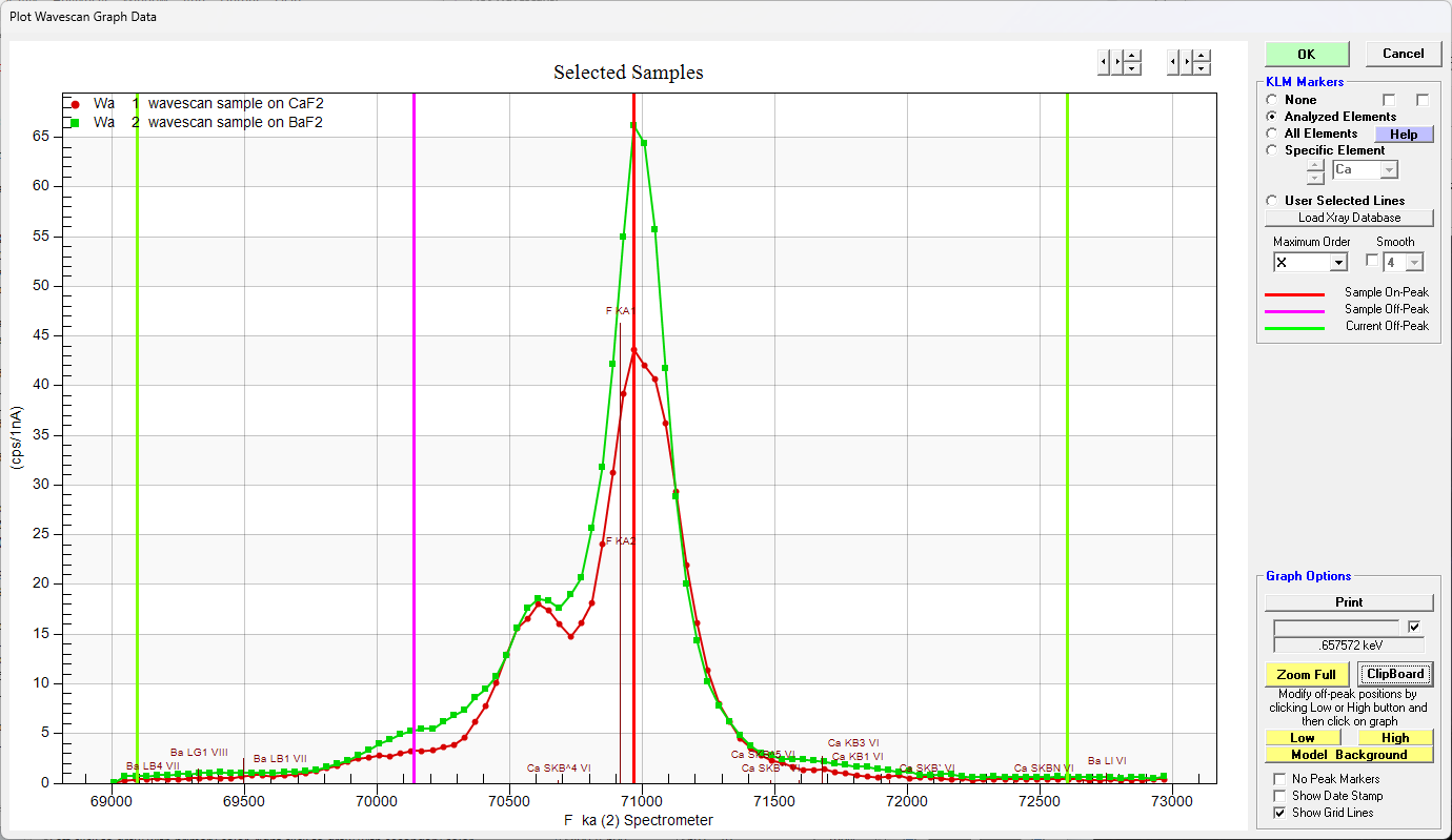
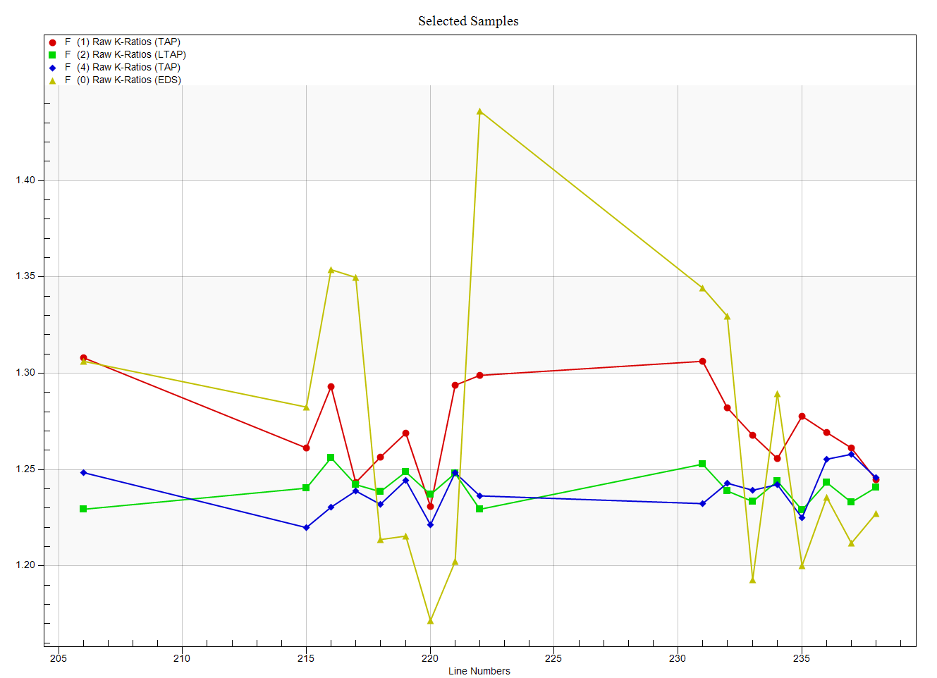
Clearly the peak intensities do not represent the integrated intensities. And in fact we can see this quite clearly when we examine the k-ratios from the EDS spectrometer and compare them to the WDS spectrometers as seen here:


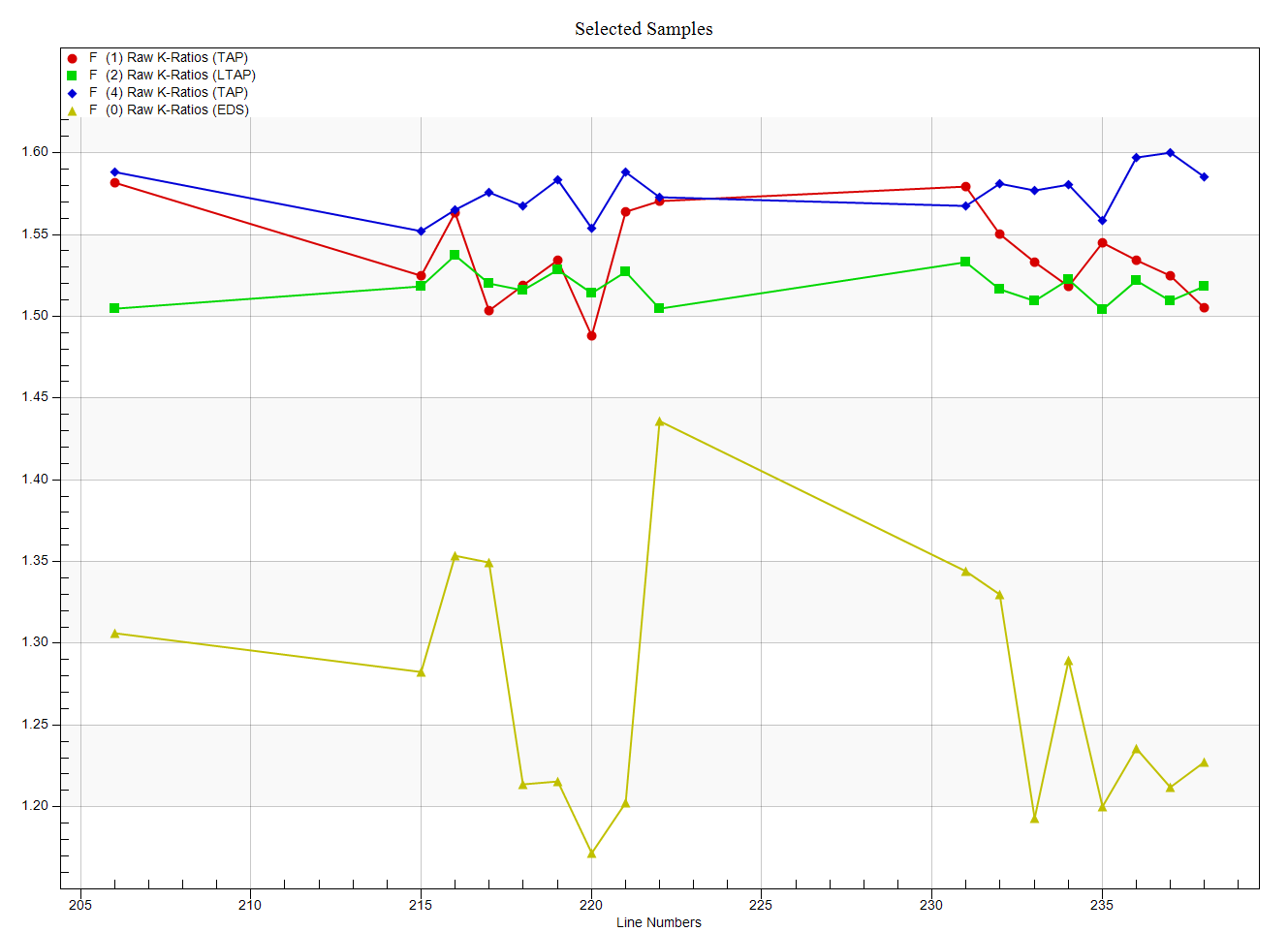
Admittedly not a great dataset, but the fact that the EDS and WDS disagree so much, I thought it might be worth looking at the Area Peak Factors (APFs) for this system a bit more. Also note that the peak position for F Ka for these two materials has not shifted, but only the peak shape.  So lets start with the CaF2 (our primary standard) using the Model Background dialog and clicking the Integrate button as shown here:


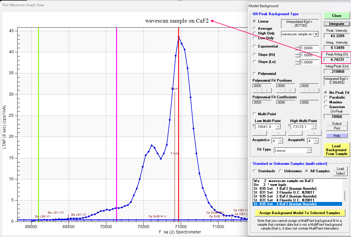
Note that we utilize the Peak/Integrated ratio for the primary standard (CaF2) and for the BaF2 (our secondary standard) we have:


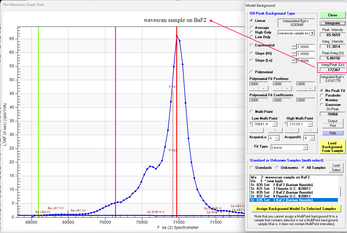
Multiplying these two values together we obtain ~0.817 or almost a 20% correction!  Applying the values calculated for each spectrometer (all three are close to ~0.80) by entering these "specified" APFs in the Elements/Cations dialog as discussed in this topic and elsewhere, we obtain the following k-ratios (the APFs are applied by Probe for EPMA automatically to the k-ratios during the matrix correction):


Which is a considerable improvement over what we had from assuming that the F Ka peak shape was unaffected by the emission matrix. Sorry for the digression, but I thought it was an interesting system to test the APF correction on...

So what does this mean for the analysis of F Ka?   Well, given this enormous peak shape correction but also the success of modeling the peak shape using APFs, one could say to use either material as the standard and use the APF correction relative to the unknown in question, as a specified APF.

But maybe it is more accurate is to use CaF2 as a primary standard for characterizing Fluor-apatites (since there is a large amount of Ca in the apatite matrix), and use BaF2 as a primary standard for fluorine in other (less absorbing) matrices.

What do you all think?   

Oh, and by the way, there is a quite large TDI correction for these materials even using a 20 um defocused beam! I will show that data in another topic also later on because I am seeing something quite odd there (what appears to be a significant difference in the TDI correction for each of the TAP spectrometers!).
« Last Edit: November 12, 2023, 03:27:55 PM by Probeman »
The only stupid question is the one not asked!