As we all know, precision is quite easy to estimate (just make some replicate measurements!), but ascertaining accuracy is more difficult and usually requires the analysis of so called "secondary" standards. These secondary standards can be any composition with a known (or zero) concentration of the element(s) of interest, but ideally they are similar in matrix (concentrations) to the unknown composition, and not assigned as a primary standard to the element(s) in question.
Evaluating accuracy for such secondary standards in Probe for EPMA is quite straight forward, since Probe for EPMA can "analyze" standards as though they were unknowns. By this I mean PFE automatically adds in elements not analyzed for (but present in the standard composition) to all standard sample acquisitions, so that the matrix correction can be calculated properly and then compared to the "published" values for that (secondary) standard as seen here:
St 305 Set 1 Labradorite (Lake Co.), Results in Elemental Weight Percents
ELEM: Na Si K Al Mg Fe Ca Mn Ti O H
TYPE: ANAL ANAL ANAL ANAL ANAL ANAL ANAL ANAL ANAL SPEC SPEC
BGDS: LIN LIN LIN MAN LIN MAN LIN LIN LIN
TIME: 30.00 30.00 20.00 30.00 30.00 30.00 30.00 20.00 30.00 --- ---
BEAM: 30.17 30.17 30.17 30.17 30.17 30.17 30.17 30.17 30.17 --- ---
ELEM: Na Si K Al Mg Fe Ca Mn Ti O H SUM
13 2.847 24.582 .112 16.343 .083 .347 9.520 .001 .026 46.823 .000 100.683
14 2.833 23.624 .101 16.355 .086 .314 9.544 -.003 .037 46.823 .000 99.714
15 2.842 23.794 .108 16.371 .078 .311 9.444 .007 -.001 46.823 .000 99.778
AVER: 2.841 24.000 .107 16.356 .082 .324 9.503 .002 .021 46.823 .000 100.058
SDEV: .007 .511 .006 .014 .004 .020 .052 .005 .019 .000 .000 .542
SERR: .004 .295 .003 .008 .002 .011 .030 .003 .011 .000 .000
%RSD: .25 2.13 5.22 .09 5.15 6.08 .55 306.38 92.79 .00 .00
PUBL: 2.841 23.957 .100 16.359 .084 .319 9.577 .000 n.a. 46.823 .000 100.060
%VAR: (-.01) .18 6.95 (-.02) -2.28 1.60 -.78 .00 --- .00 .00
DIFF: (.00) .043 .007 (.00) -.002 .005 -.074 .000 --- .000 .000
STDS: 305 358 374 305 12 395 358 25 22 --- ---
In the above example this labradorite standard (#305) is the primary (assigned) standard for Na and Al and is a secondary standard for the remaining elements. The line labled AVER: is the acquired analysis for the standard, the line labeled PUBL: is the expected analysis from the standard composition database and the line labeled %VAR is the relative percent error from the published concentration value.
Immediately it is evident that Si measured in labradorite (std #305), relative to diopside (std #358), is accurate to around several tenths of a percent, and Ca in labradorite relative to diopside again is accurate to better than a percent relative. The remaining minor and trace elements can also be examined to ascertain the ability to measure low (or zero) concentrations with his setup.
In CalcZAF, every sample is considered an unknown, so determining accuracy is slightly more work, but that simply means that one must import the analysis of a secondary standard and compare the results to the expected concentrations.
We might call this method of determining accuracy by using secondary standards an "external" method since we are checking ourselves using an external (secondary) standard. But there is another way to estimate accuracy, though secondary standards should always be acquired if at all possible!
I'll call this other accuracy assessment method an "internal" method, since we will be relying not on secondary standards, but on multiple matrix corrections. This is reason that John Armstrong called his off-line analysis program TRYZAF. Using it, one can "try" many different matrix corrections on the same dataset. This also true for CalcZAF.
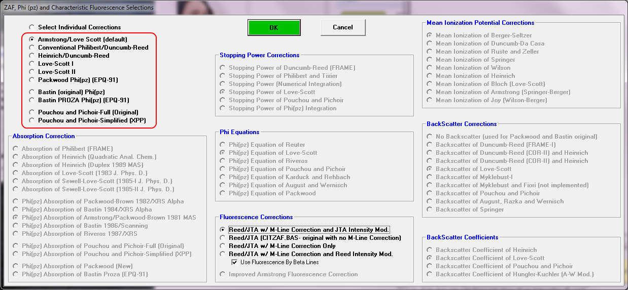
Of course we might hope that these multiple matrix correction methods will always give the same answer, but of course they don't (that's science for you!). In any case, by "internal" I simply mean we can analyze the unknown composition using a number of matrix corrections methods that are available in TryZAF, CalcZAF (and PFE of course) as seen here:
For example here is the previous labradorite (#305) composition exported from PFE and analyzed using CalcZAF with the Use All Matrix Corrections checkbox checked:
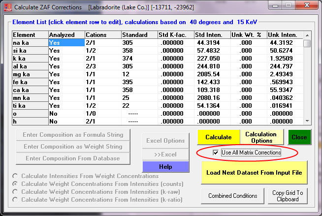
After clicking the Calculate button, we wait for the app to cycle through all 10 matrix corrections (of course all these matrix correction methods are utilizing the same mass absorption coefficient (MAC) table, so that is another parameter that can be tested. CalcZAF (and PFE) can utilize 5 different MAC tables.
Summary of All Calculated (averaged) Matrix Corrections:
Labradorite (Lake Co.)
LINEMU Henke (LBL, 1985) < 10KeV / CITZMU > 10KeV
Elemental Weight Percents:
ELEM: Na Si K Al Mg Fe Ca Mn Ti O H TOTAL
1 2.841 24.002 .107 16.356 .082 .324 9.502 .002 .021 46.823 .000 100.060 Armstrong/Love Scott (default)
2 2.840 24.109 .107 16.353 .081 .331 9.519 .002 .021 46.823 .000 100.186 Conventional Philibert/Duncumb-Reed
3 2.840 24.036 .107 16.354 .082 .319 9.498 .002 .021 46.823 .000 100.082 Heinrich/Duncumb-Reed
4 2.840 24.057 .107 16.354 .082 .324 9.505 .002 .021 46.823 .000 100.115 Love-Scott I
5 2.841 24.006 .107 16.356 .082 .324 9.504 .002 .021 46.823 .000 100.065 Love-Scott II
6 2.840 24.089 .107 16.353 .080 .329 9.532 .002 .021 46.823 .000 100.176 Packwood Phi(pz) (EPQ-91)
7 2.838 24.316 .107 16.340 .082 .322 9.620 .002 .020 46.823 .000 100.470 Bastin (original) Phi(pz)
8 2.842 23.871 .107 16.362 .080 .329 9.510 .002 .021 46.823 .000 99.947 Bastin PROZA Phi(pz) (EPQ-91)
9 2.839 24.147 .107 16.350 .082 .330 9.525 .002 .021 46.823 .000 100.226 Pouchou and Pichoir-Full (Original)
10 2.840 24.116 .107 16.352 .082 .330 9.529 .002 .021 46.823 .000 100.201 Pouchou and Pichoir-Simplified (XPP)
AVER: 2.840 24.075 .107 16.353 .082 .326 9.524 .002 .021 46.823 .000 100.153
SDEV: .001 .115 .000 .005 .001 .004 .036 .000 .000 .000 .000 .139
SERR: .000 .036 .000 .002 .000 .001 .011 .000 .000 .000 .000
MIN: 2.838 23.871 .107 16.340 .080 .319 9.498 .002 .020 46.823 .000 99.947
MAX: 2.842 24.316 .107 16.362 .082 .331 9.620 .002 .021 46.823 .000 100.470
For this particular example, the variance of the 10 matrix correction methods is quite small, so if we are having accuracy issues it is not due to the matrix correction method selected!
However, other compositions will yield quite different results for the different matrix correction methods as seen here:
Summary of All Calculated (averaged) Matrix Corrections:
St 20 Set 1 ThSiO4 (Huttonite)
LINEMU Henke (LBL, 1985) < 10KeV / CITZMU > 10KeV
Elemental Weight Percents:
ELEM: Si Zr Th O TOTAL
1 9.191 -.069 70.784 19.746 99.652 Armstrong/Love Scott (default)
2 7.713 -.062 71.150 19.746 98.546 Conventional Philibert/Duncumb-Reed
3 8.634 -.065 71.467 19.746 99.782 Heinrich/Duncumb-Reed
4 8.334 -.064 71.395 19.746 99.410 Love-Scott I
5 8.370 -.064 71.400 19.746 99.452 Love-Scott II
6 7.253 -.059 71.034 19.746 97.973 Packwood Phi(pz) (EPQ-91)
7 9.212 -.069 71.556 19.746 100.444 Bastin (original) Phi(pz)
8 8.779 -.066 71.501 19.746 99.958 Bastin PROZA Phi(pz) (EPQ-91)
9 8.365 -.065 71.396 19.746 99.442 Pouchou and Pichoir-Full (Original)
10 8.170 -.063 71.344 19.746 99.196 Pouchou and Pichoir-Simplified (XPP)
AVER: 8.402 -.065 71.303 19.746 99.385
SDEV: .608 .003 .241 .000 .701
SERR: .192 .001 .076 .000
MIN: 7.253 -.069 70.784 19.746 97.973
MAX: 9.212 -.059 71.556 19.746 100.444
Now someone might ask: OK, which matrix correction method is correct? And the answer of course is "why all of them"! At least that is what their authors will claim!
But in fact we know (or should know!), that some matrix corrections perform better for large absorption corrections, some matrix corrections work well for large atomic number differences, etc, etc etc... but none are "universal" yet!
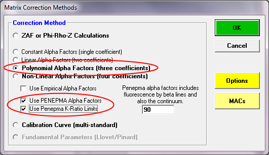
But if I wanted to hedge my bets, I would certainly utilize the Penepma alpha factor correction method. It's as good as our our current understanding of the electron solid physics involved. To run your analyses using Penepma, simply select the polynomial or non-linear alpha fit method and then check the Penepma boxes as seen here:
The results from the Penepma alpha factor method is seen here:
ELEMENT si ka zr la th ma O Total
UNK KRAT .0684 -.0005 .6500
UNK WT% 9.088 -.065 71.585 19.746 100.354
UNK AT% 17.346 -.038 16.538 66.155 100.000
UNK BETA 1.3291 1.2013 1.1014
ALPITER 5.0000
This compares well to the ideal composition for ThSiO4:
ELEM: Si Zr Th SUM
PUBL: 8.665 n.a. 71.589 100.000


 Welcome to the Probe Software forum area!