Negative Values

[mderrico]

I recently ran spinels inabyssal peridotites. I used the method of collecting off-peak and on-peak counts.
Under Elements/Cations in Analysis! I used the linear off peak correction method for my unknowns and standards. I noticed TiO2 wt% are about 70% negative values.

Is this a result of the wrong background windows being set? Also, would it be acceptable to publish data that use a high-only off peak correction for Ti for the unknowns?

The only difference I can see in my Rutile standard is that the beam current (set at 20 nA) increased on the last standard run to 30 nA.

Any suggestions or input is greatly appreciated. Thank you so much,

[John Donovan]

Negative values for intensities (KRAW) or concentrations usually indicate a problem with the background correction. Most often one or both off-peak positions are being interfered with by the presence of another x-ray line resulting in a background which is higher than the on-peak measurement.

To avoid this, it is *always* desirable to run a careful wavescan with similar precision to your on peak measurements to check for off-peak interferences. Probe for EPMA can correct for on peak interferences, but off-peak interferences must be avoided.

In a pinch, a single side background can be utilized but not if the background is sloped and it usually is except at very high sin theta spectrometer positions.

Another possible issue is that although the default off-peak interpolation method is linear, the actual shape of the background is more closely modeled using an exponential interpolation.  This option is found in the Elements/Cations dialog for each element and the actual fit can be calculated and displayed for each element in the Plot! wavescan dialog using the Model Background button.

Though normally this is not a problem except for trace elements or where the shape of the background is highly curved, e.g., low sin theta positions on the spectrometers.

For ultra trace levels certain artifacts in the continuum can produce "holes" or "negative peaks" in the continuum. This is documented for Ti ka in SiO2 for certain PET crystals (see Donovan, et. al. Am. Min, 2011). http://epmalab.uoregon.edu/pdfs/3631Donovan.pdf

In these cases a "blank" correction must be applied using the Standard Assignments dialog Blank Correction option.

The other (more fancy) method is to utilize the multi-point background (MPB) method of Jercinovic, Allaz and Donovan which is nicely implemented in PFE. This method is essentially acquiring a high precision wavescan with very few points and the quant intensities at the same time using similar precision.  The program then automatically selects the best off-peak intensities to use for the fit.

http://www.probesoftware.com/download/Poster%20EMAS%20Allaz%202011%20final.pdf

[JohnF]

As John Donovan said, you should always run wavescans around your analytical peaks, at least once for a given mineral type, so that you "learn" what may be lurking in the bushes.
 _never_ trust "book" values for background offsets, particularly if passed second or third hand, as typos and errors can occur.  Also did you check your PHA settings? What are you doing with your Ar-escape peak? are you including all of it? or excluding it? That probably is not the source of your issue, but many users are not always clear about how and when to run PHA scans (and whether or not to use differential versus integral mode). You asked is it OK to use a single background in published data. YES! If you know what you are doing! It is not always correct to use backgrounds on both sides of a peak _if you don't check for background interferences_.  My advice is not to assume anything.... I always take background for Al and Si Ka of my silicates on the positive background side (two measurements, averaged) because there is so much "x-ray traffic" on the low side of these two peaks (satellites, Kb, 2nd and 3rd order interferences from other elements in common silicate minerals and glasses).

[Julien]

I think John and John gave you here a pretty full answer. Just my two cents here...

Yes, background curvature can be pretty strong, AND you can have these "negative peak" or "hole in the background" when acquiring Ti K-alpha on PET crystal. However, you might also try to analyze Ti using a LiF crystal. Background should be a little more linear, and you probably won't have this "hole in the background" effect. The problem with LiF, of course, is that the count rate decrease quite dramatically. So it depends what range of Ti you are looking for, if this is a trace element (100 ppm or so), you might want to stick with PET crystal.

Still, getting a careful WDS scan over the area of interest around the peak is a good idea - or, should we say, a NECESSARY step especially when dealing with minor / trace element. I used to scan my samples for trace or minor elements at high current (100-200 nA) over an area covering at least 6000 *10-5 sin-theta (or 16-17 mm on JEOL) with a step of 10 * 10-5 sin-theta (or 0.035 mm on JEOL) and a counting time of 1.5 second on each step; if you can afford it (homogeneous and large sample), increase your beam diameter to 10-20 um or even more, as such scan can last for an hour or so... With this you should have a clear idea of what is in your sample and the exact shape of the background. You can then use the Plot! window in Probe for EPMA to fit a background with an optimum exponential curve (or polynomial). The multipoint background is ideal, as getting 4 or more background points will automatically fit your background curvature very accurately.

Make sure to perform a similar scan in a Ti-free standard, so you can evaluate / observe any possible "hole in the background" if you are using a PET crystal. Careful when you are performing such scan on your standard, you might want to decrease the current or increase the beam diameter further to avoid any disastrous beam/sample damage...

Julien

[mderrico]

Hi everyone,

Thank you for the feedback. I've ran a wavescan on Ti on an unknown (attached).
I did not expect any off-peak interferences, but I wanted to find out what the backgrounds looked like.

[John Donovan]

As you can see from your very nice plots, the exponential background fit works significantly better. Don't forget, your wavescan is much lower precision than your point analyses, so if you're seeing problem with a linear fit in the wavescan, it's definitely going to be a problem with your point analyses!

Did using an exponential fit help? Remember you can "adjust" the exponent of the exponential fit here for a better fit to the wavescan- when you only have two points to fit, what else can you do?   





Of course, that is exactly why we developed the "multi-point" off-peak background method. The cool thing about the multi-point background (developed by Mike Jercinovic, Mike Williams, Julien Allaz and I), is that it not only will provide the most rigorous fit for the actual background shape (because it uses more than two points, usually 4 on each side of the peak, so curvature is measured rather than assumed), but with the same precision as your unknown!

In other words, the multi-point background is sorta of like combining your wavescan *and* analysis acquisitions together!  Here is more info on the multi-point background method:

http://probesoftware.com/smf/index.php?topic=56.msg218#msg218

[mderrico]

Yes, I have concluded that for spinels, which have such low Ti, that I should use the exponential fit. For all else, I will still use linear background fits because the peaks are higher and the backgrounds are obvious.
Thank you for the tip on using the exponent of the exponential fit to see what happens to the final values.
 
What is the detection limit of the microprobe? Ti is very low in spinels and may be getting close to this limit, and depending on how background is measured, it produces the negative values. When I go to publish these values, I will assume negative values are essentially zeros. It would be helpful to know if the 0.01-0.1 wt % values are actually usable numbers given my wavescan.

Thanks!

[Probeman]

What is the detection limit of the microprobe?

What a terrific question!  So if no one minds, I'd like to take a crack at this...

Of course, the typical "scientific" answer is "it depends". Which isn't very helpful, so instead we can ask, "On what does the detection limit of the microprobe depend?"  And that is where it gets interesting... so rather than simply provide some rough numbers as is usually done, e.g., EDS 1000 PPM, WDS 100 PPM, let's determine the actual detection limit of our measurement by investigating the physics, and here are some of the "usual suspects":

1. Electron energy: generally the higher the primary (incident) beam energy, the larger the interaction volume because the higher energy electrons travel further than lower energy electrons and thus interact with more atoms before their energy drops below the critical excitation energy of the emission line under observation.  This is why many trace element analyses are performed at 20, 25 or even 30 keV.  It's the usual tradeoff between spatial resolution and sensitivity!

Exception: for many low energy emission lines, increasing the electron beam energy will cause an apparent decrease in the x-ray intensity because at very high over voltages, that is, the electron beam energy divided by the emission line critical ionization edge energy (Eo/Ec), the efficiency of ionization decreases with increasing overvoltage. In addition, very low energy emission lines will often only be emitted (as opposed to generated) from a volume very close to the sample surface due to matrix absorption, so increasing the interaction volume by increasing the electron beam energy does not improve the detection limit for these low energy emission lines such as, oxygen, nitrogen, carbon, etc.

2. Beam current: Obviously increasing the electron dosage increases the number of ionization in a linear way. Statistically speaking, doubling the beam energy will (all other considerations aside, such as sample damage), typically increase the detection limit by the square root of two (think about it!).

3. Geometric efficiency: using a larger Bragg crystal is approximately an increase in the diffraction surface area.  Using a spectrometer with a smaller focal circle is essentially subtending a larger collection angle and both methods will improve the sensitivity of the measurement.

Another method which can be used in addition to the above methods, is to simply count on multiple WDS spectrometers and combine the photons for both the on and off-peak measurements for the unknown (and also combine the on and off-peak photons for the standard as well). This is called the "aggregate" method in Probe for EPMA and is described in this paper:

http://epmalab.uoregon.edu/pdfs/3631Donovan.pdf

4. Matrix absorption: This was already mentioned, but is important that we include this effect in the calculation of detection limit, because as we lose photons to absorption, so does our sensitivity decrease. Lose half the photons because they don't escape from the sample due to photo-absorption, and we need to count twice as long. This effect can be approximated by including the matrix correction in the sensitivity calculation.

5. Counting statistics: Obviously since photon production is a quantum process we need to apply statistical considerations to the sensitivity calculation. If you only count long enough to either see or not see a photon, we have a lot of uncertainty to deal with. 

Fortunately photon counting statistics, although technically Poisson distributions (especially at very low count rates), is approximated by Gaussian (normal) statistics at reasonable count rates.

I'm leaving out a few other factors, but let's put these together in a typical detection limit calculation, this one from Goldstein et al. and is described as: a single point detection limit calculation based on the standard counts and the unknown background counts and including the magnitude of the ZAF correction factor. The calculation is adapted from Love and Scott (1983). This detection limit calculation is useful in that it can be used even on inhomogeneous samples and can be quoted as the detection limit in weight percent for a single analysis line with a confidence of 99% (assumes 3 standard deviations above the background).



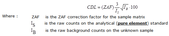
So a few of the factors described above are included here nicely. We have the ZAF matrix correction term (which could be any matrix correction such as Phi-rho-z, alpha-factors, etc.), the square root of the background intensity approximates the statistical variance, the factor 3 gives us 3 sigma statistics, the standard intensity normalizes this to concentration and times 100 gives us weight percent.

What does this look like in practice?

Well here's a typical major element analysis of a silicate glass standard in Probe for EPMA, acquired as a standard, *but* analyzed as an unknown.

St  160 Set   7 NBS K-412 mineral glass, Results in Elemental Weight Percents
 
ELEM:       Na      Si       K      Al      Mg      Ca      Ti      Mn      Fe       P      Cr       O       H
TYPE:     ANAL    ANAL    ANAL    ANAL    ANAL    ANAL    ANAL    ANAL    ANAL    ANAL    ANAL    SPEC    SPEC
BGDS:      MAN     MAN     LIN     MAN     MAN     MAN     LIN     LIN     MAN     EXP     LIN
TIME:    20.00   15.00   20.00   20.00   30.00   40.00   10.00   10.00   30.00   20.00   15.00
BEAM:    19.80   19.80   19.80   19.80   19.80   19.80   19.80   19.80   19.80   19.80   19.80

ELEM:       Na      Si       K      Al      Mg      Ca      Ti      Mn      Fe       P      Cr       O       H   SUM 
   365    .037  21.171    .007   4.808  11.703  10.870   -.009    .050   7.870    .015    .012  43.597    .000 100.131
   366    .044  21.212    .012   4.798  11.704  10.860    .014    .062   7.635    .008    .009  43.597    .000  99.955
   367    .042  21.316    .016   4.822  11.640  11.073    .011    .069   7.697    .018    .004  43.597    .000 100.305

AVER:     .041  21.233    .012   4.809  11.682  10.934    .005    .060   7.734    .014    .009  43.597    .000 100.130   <-- measured
SDEV:     .004    .075    .004    .012    .037    .120    .013    .010    .122    .005    .004    .000    .000    .175
SERR:     .002    .043    .003    .007    .021    .069    .007    .006    .070    .003    .002    .000    .000
%RSD:     8.65     .35   37.11     .25     .31    1.10  244.23   16.27    1.57   37.98   45.58     .00     .00

PUBL:     .043  21.199    n.a.   4.906  11.657  10.899    n.a.    .077   7.742    n.a.    n.a.  43.597    n.a. 100.120   <-- published or accepted
%VAR:    -4.53     .16     ---   -1.97     .21     .32     ---  -21.55    -.10     ---     ---     .00     ---
DIFF:    -.002    .034     ---   -.097    .025    .035     ---   -.017   -.008     ---     ---    .000     ---
STDS:      336     162     374     336     162     162      22      25     162     285     396       0       0

STKF:    .0735   .2018   .1132   .1331   .0568   .1027   .5547   .7341   .0950   .1599   .3050   .0000   .0000
STCT:   2517.1  9998.1  5423.2  8306.3  2850.4   337.0  6456.1 14052.2   600.2  9598.3  5218.7      .0      .0

UNKF:    .0002   .1624   .0001   .0328   .0777   .1011   .0000   .0005   .0653   .0001   .0001   .0000   .0000
UNCT:      7.1  8047.5     5.2  2044.3  3904.0   331.7      .5     9.6   412.5     5.9     1.3      .0      .0
UNBG:     11.0    10.8    29.1    26.7    19.4     1.4     5.3    18.1     7.6    37.8    12.4      .0      .0

ZCOR:   1.9912  1.3072  1.0956  1.4679  1.5026  1.0818  1.1827  1.2047  1.1841  1.3989  1.1586   .0000   .0000
KRAW:    .0028   .8049   .0010   .2461  1.3696   .9844   .0001   .0007   .6872   .0006   .0002   .0000   .0000
PKBG:     1.64  742.73    1.18   77.63  201.78  235.18    1.10    1.54   55.21    1.16    1.11     .00     .00
INT%:     ----    ----    ----    ----    -.08    ----    ----    ----     .00    ----    ----    ----    ----

Detection limit at 99 % Confidence in Elemental Weight Percent (Single Line):

ELEM:       Na      Si       K      Al      Mg      Ca      Ti      Mn      Fe       P      Cr
   365    .016    .008    .014    .010    .009    .023    .028    .031    .035    .016    .027
   366    .016    .008    .015    .010    .009    .023    .027    .033    .035    .018    .027
   367    .016    .008    .014    .010    .009    .023    .027    .029    .035    .016    .029

AVER:     .016    .008    .014    .010    .009    .023    .027    .031    .035    .017    .028
SDEV:     .000    .000    .000    .000    .000    .000    .001    .002    .000    .001    .001
SERR:     .000    .000    .000    .000    .000    .000    .000    .001    .000    .000    .001

Because all the measured elements were assigned to other standards (primary standards), the accuracy can be compared as seen in the AVER: and PUBL: lines.  But for detection limits we will examine the section just above which is based on the equation already discussed.

The detection limit for each analysis line is printed along the average and variance of the detection limits. As one can see the detection limits range from 0.035 (350 PPM) for Fe to 0.008 (80 PPM) for Si. of course we really only care about the trace elements and they vary from 0.027 (270 PPM) for Ti to 0.016 (160 PPM) for Na.

Remember, these are 3 sigma calculations so they can be quoted to 99% confidence. What if the concentration measured is higher than the quoted 3 sigma detection limit? Well it means that the confidence of detection is *better* than 99%, say maybe 99.9% confidence. And if the concentration is below the 3 sigma detection limit, what does that mean? Well it means that we have less than 99% confidence of detection, say maybe 95% confidence.

For more information on using this calculation see the attachment below (remember to login to see attachments) from Karsten Goemann's most recent rewrite of the PFE Advanced Topics manual starting on page 116.

For more information on correcting negative values using a "blank correction" see this thread here:

http://probesoftware.com/smf/index.php?topic=29.0

and also check out the PPT slide attached below and this thread on quant trace element mapping in CalcImage:

http://probesoftware.com/smf/index.php?topic=107.0

[pgopon]

Short answer the detection limit for the probe is determined by the ability to measure something as distinct from the background.  PfEPMA does provide a way for you to easily calculate your detection limit for your setup (as described in the previous post), see figure below.  Basically the longer you count with more current the better your detection limit, we have been able to get down to 5 of ppm detection limit, counting for half an hour with 100nA  using four spectrometers for measure the element of interest (Sc in our case). 

phil