Lots of great posts here. I really enjoyed reading this topic.
I looked at Sem-geologist’s MC code some time ago. I am not an expert in Python so I may have misunderstood some of it. In the function “detector_raw_model” an array of 1 million values is returned, each value representing the number of photons hitting the detector in a 1 µs interval. However, these values seem to be generated using purely random numbers (a flat distribution), not following a Poisson distribution. Is that correct? I would have expected the number of photons hitting the detector to follow a Poisson distribution and to be a function of the aimed count rate and the timing interval.
Below I will try to present the Monte Carlo code I wrote, as best as I can. I would love any feedback on it or any correction if I made a mistake.
The algorithm I wrote is very basic and does not attempt to model a physical detector. It assumes the detector is either available to detect a photon or is dead. The detector can switch from one of these two states to the other without any time delay. Once the detector is dead, it stays dead for a time equals to the dead time. This dead time is non extensible, i.e., if a new photon hit the detector while being dead, this does not extend the dead time. I assumed the emission of photons to follow a Poisson distribution. It is generally well accepted that photon emission can be described by such a distribution: the probability that k photons reach the detector in the time interval ∆t (in sec) is given by:
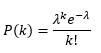
where λ=N×∆t is the average number of photons reaching the detector in the time interval ∆t and N is the emitted (real) count rate in c/s.
The Monte Carlo algorithm works with four parameters: the number of steps simulated, a time interval (∆t) corresponding to the time length of each simulated step, in second, the count rate (N) of emitted photons reaching the detector, in count per second, and the detector dead time (τ), in second. Here is the logigram (flowchart) of the code:
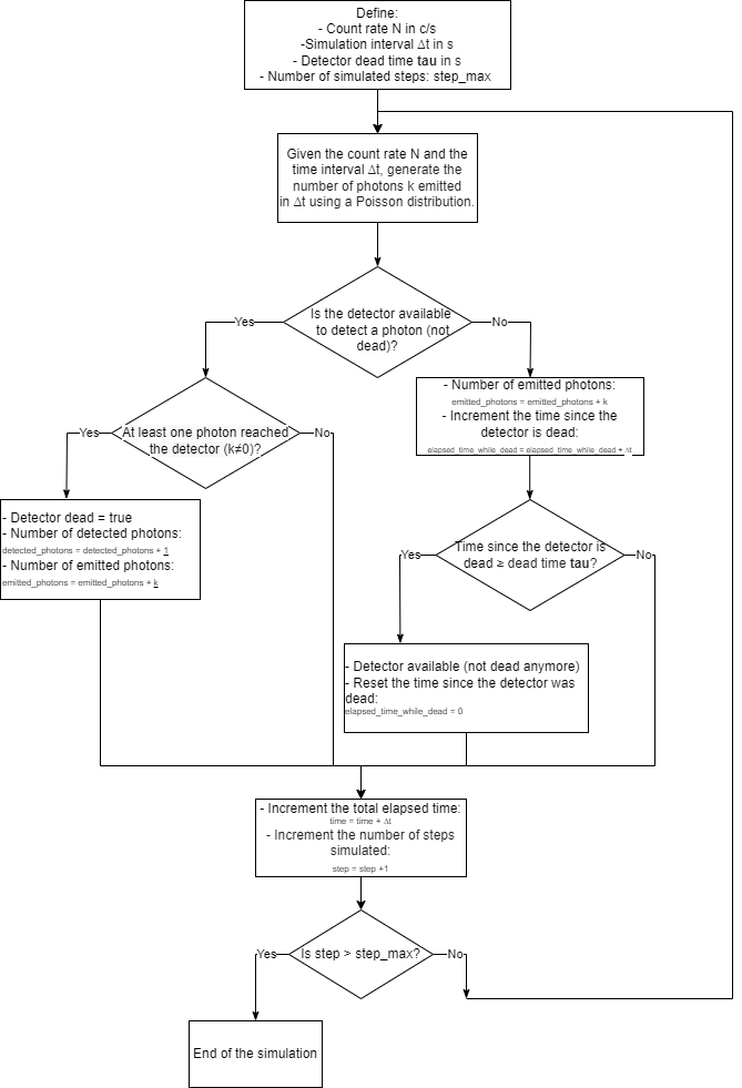
For each step of the simulation, a time interval ∆t is considered. Based on the count rate N and the time interval ∆t, the program simulates how many photons (k) are reaching the detector in this time interval using the Poisson distribution and random numbers. What I called photon coincidence is when more than 1 photon reached the detector in the time interval ∆t. Obviously, ∆t needs to be small enough compared to the detector dead time. In my simulations, I used ∆t=10 ns.
When at least one photon reaches the detector, the total number of detected photons is increased by one (only one photon at a time is detected) and the total number of emitted photons increases by k. As a result of the detection of a photon, the detector becomes dead for a period corresponding to the deadtime τ. The detector is then staying dead for a number of steps j=τ/∆t. During each of these j next steps, the program simulates how many new photons are reaching the detector. If any, these photons are not detected (because the detector is dead) but they are accounted for by the program in a variable tracking the total number of emitted photons. After j steps have passed, the detector is ready to detect a new photon. The process is repeated until the specified number of steps has been simulated.
Note that for the simulation to give realistic results, the time interval ∆t must be much smaller than the detector deadtime τ (ideally 100 to 1000 times smaller) and ∆t must be a multiple of τ.
I coded this algorithm in VBA and included it in the attached Excel spreadsheet. For a given number of simulation steps, targeted count rate, detector dead time and simulation time interval (∆t), the first spreadsheet will calculate the number of emitted photons (photons hitting the detector), the number of detected photons as well as the corresponding count rates.
The second spreadsheet will do the same but for targeted count rates of 100, 1000, 10000, 25000, 50000, 100000, 200000 and 500000 cps. The results will also be compared to the traditional dead time correction formula and plotted together. It takes about 8 seconds on my computer to simulate 30,000,000 steps and so about 1 minute to simulate the 8 targeted count rates above (the spreadsheet may seem frozen while calculating).
I was very surprised to see that this Monte Carlo code, which deals with multiple photon coincidence, gives the same results as the traditional dead time correction.

 To see the latest forum posts scroll to the bottom of the main page and click on the View the most recent posts on the forum link
