Carbon quant in steel

[Probeman]

An issue that I have also run into when measuring carbon (and nitrogen) in cross section near a surface edge is due to rounding of the sample edge where the steel meets the mounting medium.  This can be mitigated by utilizing a "surround" of a similar material hardness to the actual sample that surrounds the sample, and prevent rounding of the edge during polishing.

Here is a nice explanation of the issue:

https://books.google.com/books?id=eP6p3zQNjDYC&pg=PA268&

The problem for EPMA (and EDS) is that because our spectrometers measure the intensity at an angle (take off angle) to the surface of the sample, if the sample surface is tilted towards or away from the spectrometer, the emitted intensity will be strongly affected, especially for low energy emissions (such as carbon, oxygen, nitrogen, etc).

I'm sure others know a lot more about these sorts of effects than I do, so please feel free to chime in.

[Probeman]

I've been continuing to work on developing a method for trace carbon in steel and I am discovering that there's more that I don't know, than I do know!   

It's quite interesting how variable these carbon contamination effects are. For example last June I was performing some carbon measurements using the TDI scanning method (replicate x-ray map frames and extrapolation to zero time on a pixel by pixel basis), and found that the carbon behaves much as we would expect as described here:

http://probesoftware.com/smf/index.php?topic=933.msg5990#msg5990

However, on some carbon point analyses in the past (2015) shown here:

http://probesoftware.com/smf/index.php?topic=48.0

and recent point analyses performed this month, I instead see a downward trend over time as seen here:



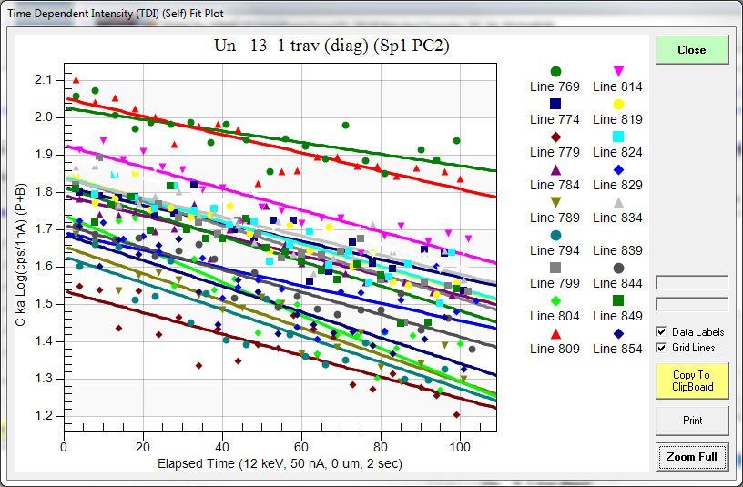
These are from a traverse of a heat treated sample displaying every 5th point. Each point is several microns apart so they should not be intersecting any carbon from a previous analysis position. Why would the carbon levels decrease over time?  The system is quite clean (we use a 100K cryo trapped system) and the sample was carefully cleaned in ethanol and dried in a 60C oven just prior to being placed in the instrument. 

Anyway, if this is of any interest to anyone, I thought I would step through the process of analyzing these samples for trace carbon and share what I have learned about characterizing trace carbon in steel.  First off, here are the results for the first 12 data points, without any specialized corrections.  That is, merely off-peak and matrix corrected results:

Un   13 1 trav (diag)
TakeOff = 40.0  KiloVolt = 12.0  Beam Current = 50.0  Beam Size =    0

Un   13 1 trav (diag), Results in Elemental Weight Percents
 
ELEM:        C       N      Al      Mo      Cr      Fe      Mn      Ni      Si       V
BGDS:      EXP     EXP     EXP     LIN     LIN     LIN     LIN     LIN     EXP     LIN
TIME:    40.00   40.00   80.00   80.00   80.00   20.00   40.00   40.00   80.00   60.00
BEAM:    50.42   50.42   50.42   50.42   50.42   50.42   50.42   50.42   50.42   50.42

ELEM:        C       N      Al      Mo      Cr      Fe      Mn      Ni      Si       V   SUM 
   769   1.561  12.073    .012   1.117   4.902  85.393    .309    .126    .858   1.342 107.693
   770   1.666  11.584    .016    .989   4.854  86.282    .348    .204    .894    .592 107.430
   771   1.018   5.889    .011   1.104   5.087  89.852    .324    .149    .950   1.121 105.506
   772    .974   5.972    .020   1.048   5.116  89.821    .358    .175    .965   1.063 105.512
   773   1.088   5.141    .016   1.015   5.085  91.173    .360    .095    .993    .661 105.625
   774   1.230   6.735    .015   1.032   5.100  88.904    .371    .108    .977    .866 105.339
   775   1.316   5.323    .013   1.070   5.165  90.751    .372    .154    .994   1.019 106.177
   776   1.054   5.001    .018   1.096   5.233  89.668    .346    .118    .984   1.401 104.920
   777    .966   5.065    .014   1.125   5.247  89.899    .330    .075    .976   1.524 105.220
   778   1.012   4.642    .012   1.010   5.167  91.519    .371    .146   1.007    .509 105.395
   779    .925   4.452    .011   1.057   5.196  91.330    .365    .163   1.023    .472 104.995
   780    .942   4.759    .008   1.158   5.237  91.516    .321    .189   1.014    .599 105.743

Pretty awful as one can see.  Oh, I guess I should show the background fits for carbon (and nitrogen), so here they are, first for carbon:



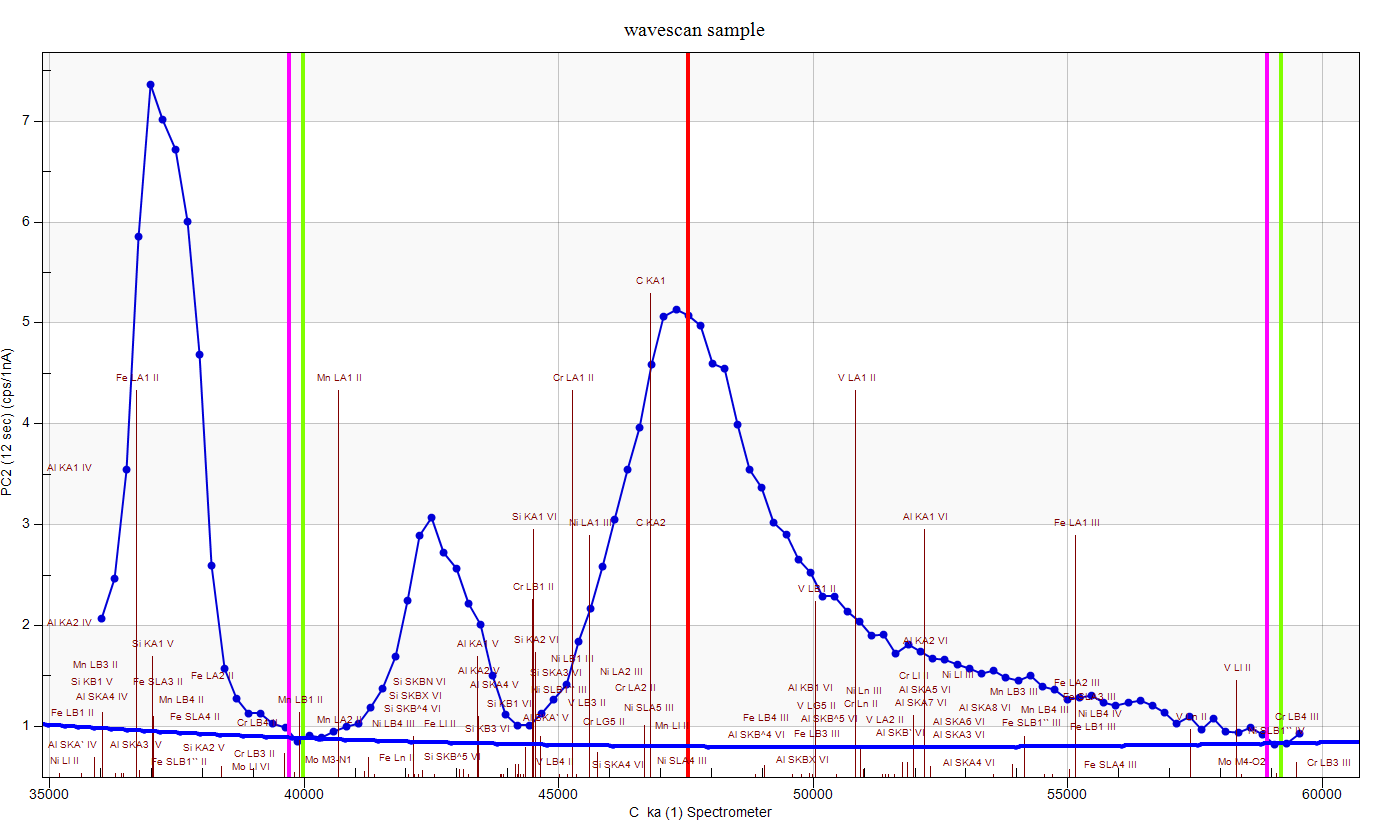
Now we can assume that are not seeing the actual carbon background here.  The tails in this region extend a long way, especially when using LDE/PC multi-layer Bragg crystals for these emission lines.  But measuring too high a background, would give us *lower* carbon results than we expect, not higher.  Either way, the blank correction should take care of it. And here are the results for the nitrogen scan:



So, now let's add in some other corrections that might be useful. Let's start with the TDI correction, which (unfortunately) we would expect to further increase our carbon concentration since we are seeing (for whatever reason!), negative slopes in our carbon TDI plots:

Un   13 1 trav (diag)
TakeOff = 40.0  KiloVolt = 12.0  Beam Current = 50.0  Beam Size =    0

Un   13 1 trav (diag), Results in Elemental Weight Percents
 
ELEM:        C       N      Al      Mo      Cr      Fe      Mn      Ni      Si       V   SUM 
   769   1.687  12.426    .012   1.124   4.905  85.939    .310    .126    .858   1.343 108.731
   770   1.825  12.013    .016   1.006   4.864  85.644    .348    .204    .894    .593 107.408
   771   1.182   5.907    .011   1.115   5.094  88.742    .324    .149    .950   1.122 104.597
   772   1.084   5.959    .020   1.049   5.117  89.920    .358    .175    .965   1.063 105.710
   773   1.364   5.181    .016   1.030   5.092  90.421    .360    .095    .993    .662 105.214
   774   1.393   6.908    .015   1.048   5.108  88.082    .372    .109    .976    .867 104.879
   775   1.570   5.366    .013   1.054   5.170  90.220    .372    .154    .994   1.020 105.933
   776   1.311   5.339    .018   1.146   5.242  89.817    .347    .118    .984   1.403 105.725
   777   1.086   5.105    .014   1.139   5.248  90.361    .330    .075    .976   1.524 105.858
   778   1.272   4.520    .012   1.017   5.165  92.675    .371    .146   1.007    .509 106.695
   779   1.070   4.407    .011   1.047   5.200  90.444    .366    .163   1.023    .472 104.204
   780   1.110   4.931    .008   1.182   5.242  91.641    .321    .189   1.014    .599 106.237

And sure enough we're seeing a small increase of carbon, for example the first data point goes from 1.56 wt.% to 1.69 wt.%.  And the average TDI parameters are here:

TDI%:   15.038   1.388   -.169    .025    ----   -.044    ----    ----    ----    ----
DEV%:      2.7     8.2     3.0     4.5    ----      .3    ----    ----    ----    ----
TDIF:  LOG-LIN LOG-LIN LOG-LIN LOG-LIN    ---- LOG-LIN    ----    ----    ----    ----
TDIT:   102.90  104.42  137.20  137.16    ----   71.79    ----    ----    ----    ----
TDII:     6.13    2.30    3.40    2.59    ----    87.2    ----    ----    ----    ----
TDIL:     1.81    .832    1.22    .952    ----    4.47    ----    ----    ----    ----

So a 15% increase in carbon at the ~1.5% wt.% level.  But why are our totals so darn high?  Well first of all, we appear to have some "native" carbon on our sample, as a "blank" measurement on pure Fe gives us about 1 wt.% carbon. Interestingly, if we look at the carbon TDI on our blank we see almost no TDI effect:



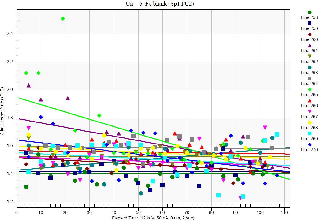
How weird is that?  Same instrument, different sample...

Now after the blank correction is applied we now obtain these quant results:

Un   13 1 trav (diag)
TakeOff = 40.0  KiloVolt = 12.0  Beam Current = 50.0  Beam Size =    0

Un   13 1 trav (diag), Results in Elemental Weight Percents
 
ELEM:        C       N      Al      Mo      Cr      Fe      Mn      Ni      Si       V   SUM 
   769    .557  12.112    .012   1.124   4.889  85.662    .309    .126    .859   1.339 106.987
   770    .696  11.708    .016   1.006   4.848  85.365    .347    .204    .895    .591 105.675
   771    .048   5.751    .011   1.115   5.077  88.448    .323    .149    .951   1.119 102.991
   772   -.051   5.802    .020   1.048   5.099  89.625    .357    .175    .966   1.060 104.101
   773    .231   5.045    .016   1.030   5.075  90.126    .359    .095    .994    .660 103.631
   774    .260   6.727    .015   1.048   5.091  87.793    .370    .108    .977    .865 103.254
   775    .439   5.227    .013   1.054   5.153  89.931    .371    .153    .995   1.016 104.352
   776    .178   5.199    .018   1.145   5.224  89.525    .346    .118    .985   1.399 104.137
   777   -.049   4.971    .014   1.138   5.230  90.067    .329    .074    .977   1.520 104.272
   778    .137   4.403    .012   1.016   5.148  92.378    .370    .146   1.008    .508 105.127
   779   -.065   4.290    .011   1.046   5.183  90.147    .364    .163   1.024    .471 102.634
   780   -.026   4.803    .008   1.181   5.225  91.344    .320    .188   1.015    .597 104.656

Now we are seeing carbon pretty much hovering around zero, but our totals are still pretty bad.  What could be going on?

Well I didn't mention this yet, but most of you probably guessed that the standards are carbon coated, but the unknown sample is *not* carbon coated- because, you know, we're trying to analyze for carbon here!   

And at 12 keV, the low overvoltage affects the Fe Ka emissions pretty strongly.  And I should also mention that this is why we should always utilize standards- because if we normalize to 100% every analysis looks perfectly fine...  So let's specify a carbon coat for the standards by checking these boxes in the Analysis Options dialog:



The standards are by default specified as 20 nm of carbon, now how do we specify no coating for our unknown sample?  We use the calculation Options dialog as seen here and simply uncheck the Use Unknown Conductive Coating correction for the sample as seen here:



And now we obtain these results, with the TDI, blank and coating corrections:

Un   13 1 trav (diag)
TakeOff = 40.0  KiloVolt = 12.0  Beam Current = 50.0  Beam Size =    0

ELEM:        C       N      Al      Mo      Cr      Fe      Mn      Ni      Si       V   SUM 
   769    .548  10.071    .012   1.093   4.714  82.164    .297    .119    .836   1.294 101.147
   770    .682   9.734    .015    .978   4.674  81.887    .334    .193    .871    .571  99.940
   771    .050   4.766    .011   1.085   4.904  84.977    .311    .141    .925   1.083  98.253
   772   -.045   4.809    .019   1.020   4.925  86.107    .344    .166    .940   1.026  99.311
   773    .226   4.180    .015   1.002   4.903  86.609    .346    .090    .967    .639  98.978
   774    .256   5.578    .015   1.019   4.915  84.323    .357    .103    .951    .837  98.354
   775    .427   4.331    .013   1.025   4.979  86.419    .358    .146    .968    .984  99.648
   776    .175   4.308    .018   1.114   5.047  86.028    .334    .112    .958   1.354  99.448
   777   -.044   4.118    .014   1.108   5.053  86.555    .317    .071    .950   1.471  99.613
   778    .136   3.647    .011    .989   4.975  88.794    .357    .139    .980    .491 100.520
   779   -.059   3.553    .011   1.018   5.008  86.649    .351    .155    .996    .456  98.137
   780   -.021   3.979    .008   1.150   5.048  87.788    .308    .179    .988    .578 100.004

Holy Toledo, that's not looking too bad!  Maybe we can actually perform trace carbon analyses after all...   

[Les Moore]

Edit by John: Moved this discussion into the carbon in steel topic

My half penneth....
I read raw X-Ray count mapping data direct into Excel.
I start fom the csv file output from the JEOL 8530F+
It works a treat.
You can setup linear calibration on the counts to create a concentration matrix.

You then use conditional formatting to set a min concentration = black and a max concentration/number to white.
Resize the cell size size to 1X1 pixels (or 2).
Copy and paste the grey scaled data into Corel Paintshop Pro (I can't speak for any other program)
You then have the grey scaled image in PSP with, courtesy of Excel knowing best, an extra pixel on the top and the LHS.
 
This allows you infinite flexibility; you could do
1. ratios of quant concs (dating)
2. Linear and non-linear functions of concentrations (CEQ, Liquidus, phase boundaries etc)
3. Thickness maps of nanofilms - who needs GDS, Auger or HRTEM.

Excel copes readily with 500x500 pixels but grinds very slowly at 1000x1000 pixels.
I suppose it's not optimized for such things but its flexibility is legend.

I enclose one done just this week. 
35mm square (1024x1024pixels) quant Ni in steel ALL done in excel.
I intend to combine the Quant Ni, Cr, Mn, Mo and Si into an IDiam map (hardenability map)
Wish me luck :-)


 
 

[Les Moore]

Hi Probeman,

Glad to see you could demagnetise your samples.

I note with some interest/concern/amazement the Nitrogen content of these steels.
Is that percent?

If so, you should have only Nitrides present at these levels and not a Martensitic steel at all.
In fact, Nitrogen is an Austenite (high temperature phase) stabilizer and you should not be able to quench these steel to Martensite.

For some of the problems you have identified, I refuse to do quant C (or N) in any steel sample.
Other things to consider....
1. The C contamination may not be laid down where the spot is; if the spot heats up the surface, it self cleans and sheds the C to  a ring around the spot.
2. If the steel truly is Martensitic then its carbon content may be inhomogeneous on a sub micron scale due to carbide formation.
3. If the steel was originally banded  i.e. ferrite and pearlite bands and the Austenising treatment of insufficient time, (homogenising at high temp) then the C distribution may be a remnant of this banding.
NB ferrite has ~0.008 wt% C at RT and Peralite ~0.8 wt% C depending on the CEQ (Metallurgical black art measurement).
   
Lastly a minor quibble... a carbon content of 0.4 and above would put the steel into a "high carbon content" range and calling this a trace level analysis may raise a few Metallurgists' eyebrows.
For steels, low carbon steels are desired to have ~20ppm C and even these few and far carbon atoms are tied up in Ti(CN).
   

[Probeman]

I note with some interest/concern/amazement the Nitrogen content of these steels.   Is that percent?

If so, you should have only Nitrides present at these levels and not a Martensitic steel at all.
In fact, Nitrogen is an Austenite (high temperature phase) stabilizer and you should not be able to quench these steel to Martensite.

Hi Les,
Thanks for the info.  Yes, there's a lot of nitrogen. I probably shouldn't call it a steel.  What would you steel dudes call an Fe alloy composition with 10% N, 1% Mo and 4.5% Cr?

ELEM:        C       N      Al      Mo      Cr      Fe      Mn      Ni      Si       V   SUM
   769    .548  10.071    .012   1.093   4.714  82.164    .297    .119    .836   1.294 101.147
   770    .682   9.734    .015    .978   4.674  81.887    .334    .193    .871    .571  99.940

As I think I mentioned, the sample is a heat treated nitrided alloy from a academic research lab, so they are expecting significant N near the edge.  But I have no idea what is normal for these materials.

The t-test values are unreliable because the composition varies from the edge, but the single point statistics are quite good:

Detection limit at 99 % Confidence in Elemental Weight Percent (Single Line):

ELEM:        C       N      Al      Mo      Cr      Fe      Mn      Ni      Si       V
   769    .043    .228    .005    .020    .011    .104    .054    .091    .005    .035
   770    .034    .222    .005    .020    .011    .123    .052    .088    .005    .038
   771    .039    .244    .005    .021    .011    .111    .055    .093    .005    .037
   772    .034    .216    .005    .020    .011    .107    .052    .090    .005    .038
   773    .034    .227    .005    .020    .011    .101    .054    .095    .005    .036

AVER:     .037    .227    .005    .020    .011    .109    .053    .091    .005    .037
SDEV:     .004    .011    .000    .000    .000    .009    .001    .003    .000    .001
SERR:     .002    .005    .000    .000    .000    .004    .001    .001    .000    .001

Percent Analytical Relative Error (One Sigma, Single Line):

ELEM:        C       N      Al      Mo      Cr      Fe      Mn      Ni      Si       V
   769     3.0     1.2    17.5     1.3      .2      .4     8.4    30.6      .4     2.1
   770     2.2     1.2    13.7     1.4      .2      .4     7.4    18.7      .4     3.9
   771    15.6     2.1    20.1     1.3      .2      .3     8.2    26.4      .4     2.4
   772  -496.4     2.0    11.3     1.3      .2      .3     7.2    22.0      .4     2.5
   773     5.0     2.3    14.3     1.4      .2      .3     7.3    41.7      .4     3.4

AVER:    -94.1     1.7    15.4     1.3      .2      .3     7.7    27.9      .4     2.9
SDEV:    224.9      .5     3.5      .0      .0      .0      .5     8.9      .0      .7
SERR:    100.6      .2     1.5      .0      .0      .0      .2     4.0      .0      .3

For me this primarily an exercise in trying to understand how carbon and nitrogen might be quantified in these matrices.  Got to love a challenge!   

Lastly a minor quibble... a carbon content of 0.4 and above would put the steel into a "high carbon content" range and calling this a trace level analysis may raise a few Metallurgists' eyebrows.
For steels, low carbon steels are desired to have ~20ppm C and even these few and far carbon atoms are tied up in Ti(CN).

I think there is little if any carbon in the matrix of this sample (except maybe for the first few points on the edge and some random others).  The variation may represent sub micron inclusions which are beyond my tungsten gun's resolving capabilities.

Someday maybe I will have access to a FEG instrument!

[Probeman]

I read raw X-Ray count mapping data direct into Excel.
I start from the csv file output from the JEOL 8530F+
It works a treat.
You can set up linear calibration on the counts to create a concentration matrix.

You then use conditional formatting to set a min concentration = black and a max concentration/number to white.

I have to ask: are these raw x-ray maps background corrected?.  If not, do all your phases have the same average Z?  Different phases will often have different average Zs and hence different zero concentration intensities, and therefore will require an actual background correction.

What about absorption, fluorescence corrections?  Interference corrections?  We have quantitative matrix corrections for a reason...   

Calibration curves have their place for sure (e.g, carbon in steel), but wouldn't a background corrected, interference corrected and matrix corrected x-ray map be more quantitative?

[Les Moore]

Looking at the phase diagram again, it would appear that you might have the Fe2N on the surface followed by an intergrowth of Fe4N into the matrix.
From the dim dark past, my memory suggests the former of these grows as a nice hard layer, the latter less so and is often seen as needles.
Beneath these 'layers', you probably have a duffusion profile that is highly compromised by enhanced diffusion down prior austenite boundaries.

The link I shared before has some informative Metallography but not technically deep:
https://vacaero.com/information-resources/metallography-with-george-vander-voort/1138-microstructure-of-nitrided-steels.html

You could try etching it and seeing the phases present; just don't map it after etching in Nital 

Lastly, you could always map first and ask questions later 

[Les Moore]

The steel is ~98%Fe and there are no significant ZAF factors.
Or, more correctly, I should say the ZAF individual factors are way way below the SE of the measurement and any of the raft of errors that can be attributed to the mapping process.

When you start to have two phases such as in stainless steels you have major issues with localised variations in Cr, Mn, Fe & Ni - then you need full correction.
When you have pearlite, a eutectoid mixture of lamellar of Fe3C and iron, the Z & A factors are a function of the scale and the angle of the colony to the surface; nasty indeed.

[Probeman]

The steel is ~98%Fe and there are no significant ZAF factors.
Or, more correctly, I should say the ZAF individual factors are way way below the SE of the measurement and any of the raft of errors that can be attributed to the mapping process.

When you start to have two phases such as in stainless steels you have major issues with localised variations in Cr, Mn, Fe & Ni - then you need full correction.
When you have pearlite, a eutectoid mixture of lamellar of Fe3C and iron, the Z & A factors are a function of the scale and the angle of the colony to the surface; nasty indeed.

Hi Les,
OK, that makes sense now.   I guess I'm asking a general question about accuracy and calibration curves.  I appreciate the power of calibration curves applied to specific situations- as I've said in the past, calibration curves account for everything one doesn't know about!   

So if one has say trace carbon standards going from zero to say, 1.2 wt% carbon in iron, then I can see how one could assign a zero value and a max value, since the standards cover the range of composition.

I can also see that if one has a background corrected map, and one assumes that the lowest pixel value is a zero concentration, then we might fix the zero concentration level, on that zero basis.  That is essentially what one is doing with a blank correction (though the blank correction in PFE has some additional flexibility in that the blank level doesn't have to be zero, and the correction is applied as an intensity correction, with a matrix correction relative to the primary standard). 

The nice thing about assigning a zero (blank) is that we can have a priori reasons for assuming zero, for instance the element is below detection from bulk techniques, but without another standard how do we assign a maximum value?

So here's my question: if one doesn't have a non-zero concentration carbon or nickel standard (as in our examples), how does one assign an upper concentration value to the "white" pixels?  I'm probably still missing something...

[Probeman]

Looking at the phase diagram again, it would appear that you might have the Fe2N on the surface followed by an intergrowth of Fe4N into the matrix.

You are most sagacious, sir! 

Un   13 1 trav (diag), Results Based on 1 Atoms of n

ELEM:        C       N      Al      Mo      Cr      Fe      Mn      Ni      Si       V   SUM 
   769    .068   1.000    .001    .016    .126   2.044    .008    .003    .041    .035   3.342
   770    .087   1.000    .001    .015    .129   2.108    .009    .005    .045    .016   3.414
   771    .023   1.000    .001    .033    .277   4.467    .017    .007    .097    .062   5.984
   772   -.001   1.000    .002    .031    .276   4.487    .018    .008    .097    .059   5.978

Lastly, you could always map first and ask questions later 

Since I know very little about these materials, that's about all I can do!