Hi,
I've written a R script to plot PFE WDS wavescans in DTSAII for viewing, which maybe useful, or at least here are the pitfalls.
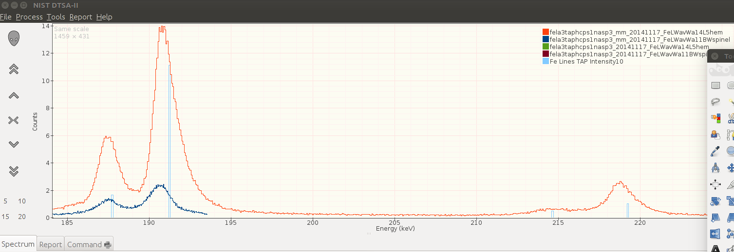
For each MDB it generates emsa and xy text files for each sample and each element/spectrometer. It also generates a ggplot for each element/spectrometer.
3 folders are created
(1) Temp - xy files
(2) L value
(3) Energy
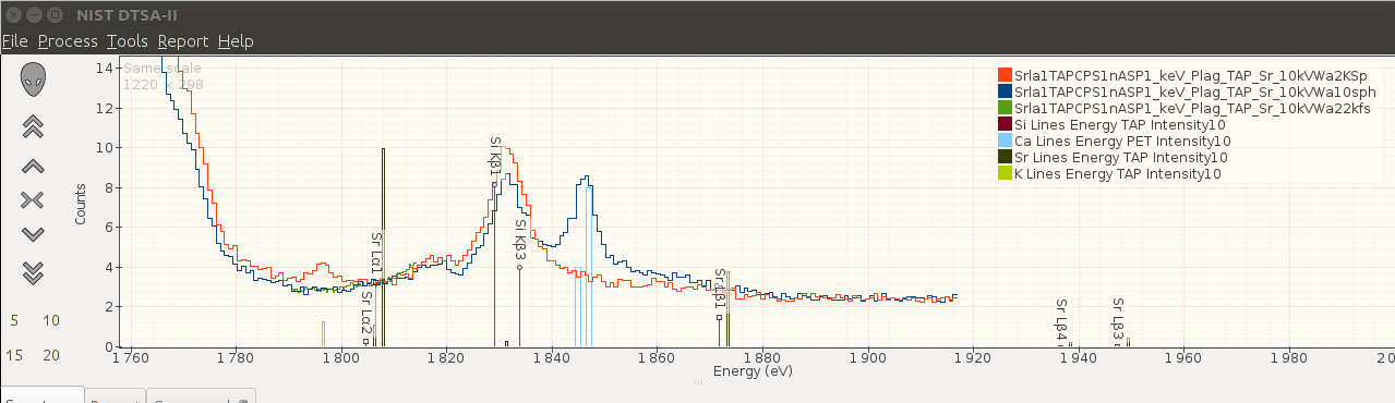
For both L value and energy I've written seperate scripts and emsa files to generate x-ray line marker spectra for the elements - the coloured columns on the graphs above. For energy the inbuilt KLM markers work but they don't include high order lines. Another quirk when viewing as energy which I didn't appreciate is that if spectra of different lengths/spacing are compared there will be a slight shift of a few eV. This is because emsa files are plot based on the step (channel) size. But when converting mm or wavelength into energy - 1 mm step does not equal a constant eV step. At the extreme's for TAP a 1mm step at 250mm = 2eV whilst at 77mm = 20eV.
For the scripts you have to set working directory (folder with MDB - and wavescans exported for each sample as dat files), location of header & footer files and location of lvalue.csv file
Ben
see attachment


 To see the latest forum posts scroll to the bottom of the main page and click on the View the most recent posts on the forum link