The goal of both methods (low keV analysis and low overvoltage analysis) is a small interaction volume, so it would be interesting to compare, say, Ni Ka at 10 keV with say, Ni La at 5 keV. One can model these scenarios with the Run | Model Xray and Electron ranges window in CalcZAF. For accurate modeling we would of course use Monte-Carlo, but this will give us some rough numbers to play with.
In this screen shot, we model Ni Ka in the NIST NiFE alloy at 15 keV. The 99% electron range is 0.94 um, but the 99% Ni Ka production range is only 0.59 um because once the incident electron energies drop below the Ni ka K edge (8.33 kV), they cannot generate inner shell ionizations thus limiting the interaction volume.
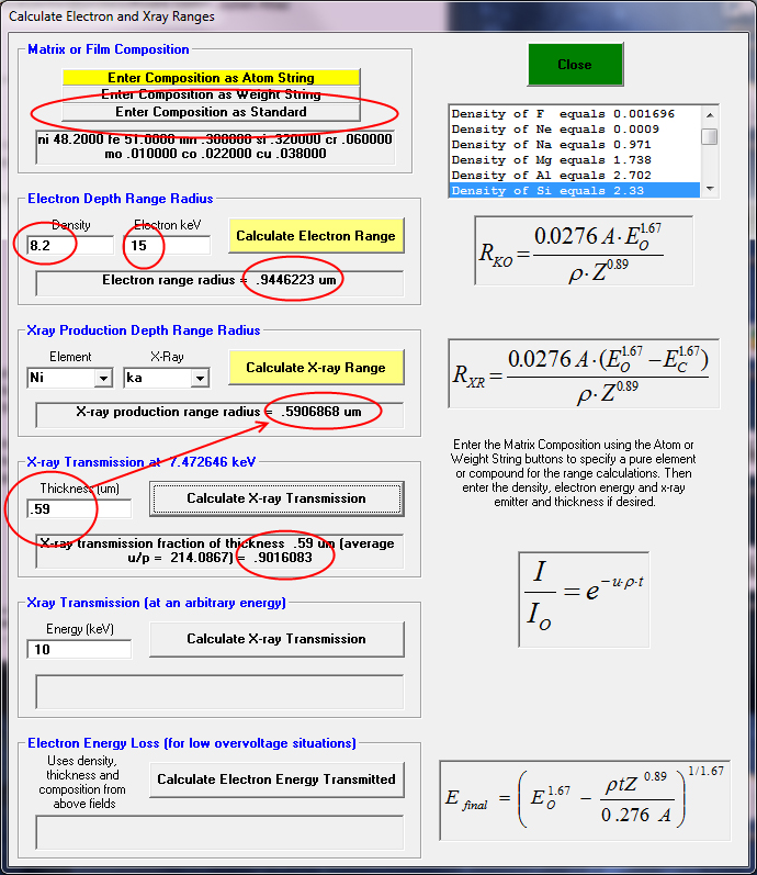
Note also the Ni ka transmission at the 99% electron depth (0.59 um) is ~90%. This will be an important number to check when we model Ni La.
The disadvantage of low overvoltage is that you might need several voltages if the various emission energies are quite different (e.g., Ni Ka vs. Si Ka). But the advantage is that one can use K lines for transition element quant, which behave better than the L lines. One the other hand, low overvoltage analysis can be problematic because the analysis can be quite affected by native oxide layers, carbon coating thickness and the physics of low overvoltage modeling.
Let's try the same analysis, now at 10 keV... We'll continue with further discussion in a moment.


 To protect your privacy, you must first log in before you can view forum statistics and user profiles