RGB overlays are a tricky subject if you look at the literature on co-localisation.
There are two approaches, the one that Ben has shown and is the implementation which has been chosen by John. This is merely plotting the pixels from more than one map onto the same space (forgive me if it is not that simple John), if they coincide then you may get some colour change but it is not consistent, it depends heavily on the concentrations of the components. If one has a higher concentration it is likely to swamp the others. If they are co-localised we need clear colour change with a range reflecting the intensity differences. This is a common problem which has been discussed in the literature. It is high dependent upon relative intensities (see http://medicine.emory.edu/documents/mimcore/bolte-guided-tour-coloc-jmrosc2006.pdf).
Merge images are being moved away from in the field of biology and various coefficients are taking their place as well as scatter plots. A lot seem to use Pearson’s image correlation coefficient. This only compares two images as far as I can tell. There is a great intro to this here: http://www.pasteur.gr/wp-content/uploads/Quantitative-Imaging-for-Colocalization-Analysis.pdf
As Dan Ruscitto pointed out he used ImageJ for this. From my previous perusing of this area it could be the best place to go. My thoughts now wander to a more philosophical discussion on what we as a community want or need. Do we want an all in one solution from John where he works on re-inventing the wheel or do we want him to work on improving our ability to collect good quality data easily and consistently which he is very good at? To my mind it may be better to request an easy output to individual quantified tiff files with headers for further processing in a programme such as ImageJ with some discussion on the forum about how we use these tools (a new section in the forum?).
Hi Gareth,
Very interesting. I did not know of this literature, but I'm not surprised of course.
And I agree, that the RGB methods that Ben and I are using are related but different. This is because the Surfer method that Ben showed is based on the transparency component, while the method I am using is, as you said, based on the more classical method of calculating the fractional components for the RGB values in the 24 bit color value. Here is the code I am using:
' Loop through all pixels in RGB channels
For ipixely& = 1 To iy&
For ipixelx& = 1 To ix&
ipixels& = ipixels& + 1
' Check for blanking value (only on first image)
If InputArray!(ipixelx&, ipixely&, 6) <> BLANKINGVALUE! Then
RGB_WtPercents!(1) = InputArray!(ipixelx&, ipixely&, R_Column%)
RGB_WtPercents!(2) = InputArray!(ipixelx&, ipixely&, G_Column%)
RGB_WtPercents!(3) = InputArray!(ipixelx&, ipixely&, B_Column%)
' Calculate composite color
If RGB_WtPercents!(1) + RGB_WtPercents!(2) + RGB_WtPercents!(3) <> 0# Then
RGB_Fractions!(1) = RGB_WtPercents!(1) / (RGB_WtPercents!(1) + RGB_WtPercents!(2) + RGB_WtPercents!(3))
RGB_Fractions!(2) = RGB_WtPercents!(2) / (RGB_WtPercents!(1) + RGB_WtPercents!(2) + RGB_WtPercents!(3))
RGB_Fractions!(3) = RGB_WtPercents!(3) / (RGB_WtPercents!(1) + RGB_WtPercents!(2) + RGB_WtPercents!(3))
' Check for range
If RGB_Fractions!(1) < 0# Then RGB_Fractions!(1) = 0#
If RGB_Fractions!(2) < 0# Then RGB_Fractions!(2) = 0#
If RGB_Fractions!(3) < 0# Then RGB_Fractions!(3) = 0#
If RGB_Fractions!(1) > 1# Then RGB_Fractions!(1) = 1#
If RGB_Fractions!(2) > 1# Then RGB_Fractions!(2) = 1#
If RGB_Fractions!(3) > 1# Then RGB_Fractions!(3) = 1#
' Save to BMP array
RGB_Color_Array&(ipixelx&, ipixely&) = RGB(CByte(RGB_Fractions!(1) * 255), CByte(RGB_Fractions!(2) * 255), CByte(RGB_Fractions!(3) * 255))
End If ' zero sum check
End If ' blanking value check
Next ipixelx&
Next ipixely&
Nothing surprising there...
And you are also correct that the highest intensity or concentration tends to dominate the RGB color. But that got me thinking about this post here:
http://probesoftware.com/smf/index.php?topic=427.msg2373#msg2373where I pointed out to Ben Buse about using the "log weight percents" to see subtle variations when you have a range of variation on different scales.
So I checked and found that although I am calculating the log wt% GRD files for display in CalcImage, I wasn't outputting the log wt% classify output .DAT file that is used for post processing. That is remedied in the latest PFE update.
So, what does that do in RGB space...? Well here's normal elemental quant wt% for an amphibole bearing basalt:
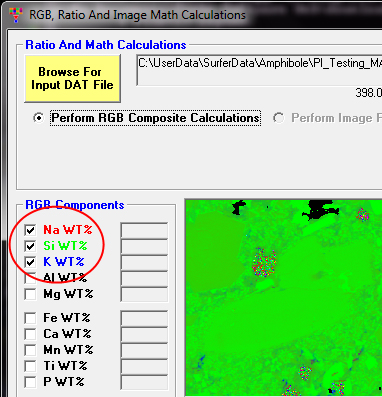
We can see that because Si is a high concentration in many pixels, and because it is assigned green in RGB space, most of the image shows as green without a lot of differentiation. Now, here is the *same* data but expressed as Log wt%:
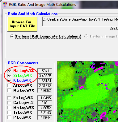
Now, let's admit it. That is a striking improvement.
I don't know if anyone else has utilized this "RGB log weight percent" technique previously, but if it hasn't been published I would be happy to work with someone to willing to write up an short abstract or poster. And I would be pleased to assist as last author if that would be helpful...


 We are a community of analysts, that cares about EPMA