Unrelated to Karsten's above post but I need to mention something disturbing I've recently become aware of.
And I should provide some examples and more detail but let me just briefly mention something about x-ray map quantification. I've recently noticed that one or two software packages are attempting quantify raw x-ray maps by using a few point analyses. The idea is to create a sort of calibration curve for relating x-ray intensities to concentrations. However, as we know from physics, the same x-ray intensity can represent very different concentrations in different phases (and visa versa). Not to mention problems with phases with different average atomic numbers and the effect of this on quantification of minor and trace element mapping.
The bottom line is that *proper* quantification of x-ray maps needs to treat *every* pixel, just as we treat our point analyses. That is every pixel needs to be treated for deadtime, background, matrix and interference corrections. Now some might say, that the precision in x-ray maps just isn't there for high accuracy quantification. I will disagree, because there's this thing called pixel averaging:
https://probesoftware.com/smf/index.php?topic=1144.msg7825#msg7825
We can have good statistics and excellent accuracy if we would only treat our x-ray map pixels just like we treat our point analyses! That is, reporting an average and a variance with each result!
I will be speaking on quantification of x-ray maps at the QMA 2019 in Minnesota later this month but wanted to add to the concerns I posted previously above with regard to utilizing calibration curves for quantification of x-ray maps.
But first consider this question: why do we *not* use such calibration curves for our point analyses? And the answer is very simply, it is generally not very accurate. That is to say, if calibration curves handled the absorption correction matrix physics well enough, we'd be using calibration curves for our point analyses. It would certainly make life for us physics modelers a lot easier!
Now there are situations where I myself would consider the use of calibration curves for quantitative analysis, assuming one has standards that are suitable for such calibrations, e.g., measuring trace carbon in steel. And occasionally one will find that a calibration curve that will work surprisingly well for a specific situation now and then, but it simply cannot be relied on for accurate quantification in general.
A case in point: geologists often analyze for silicate and oxide minerals, and here is an example of such a calibration curve (which can be selected in Probe for EPMA as an analytical method), for Mg in various oxides and silicates:
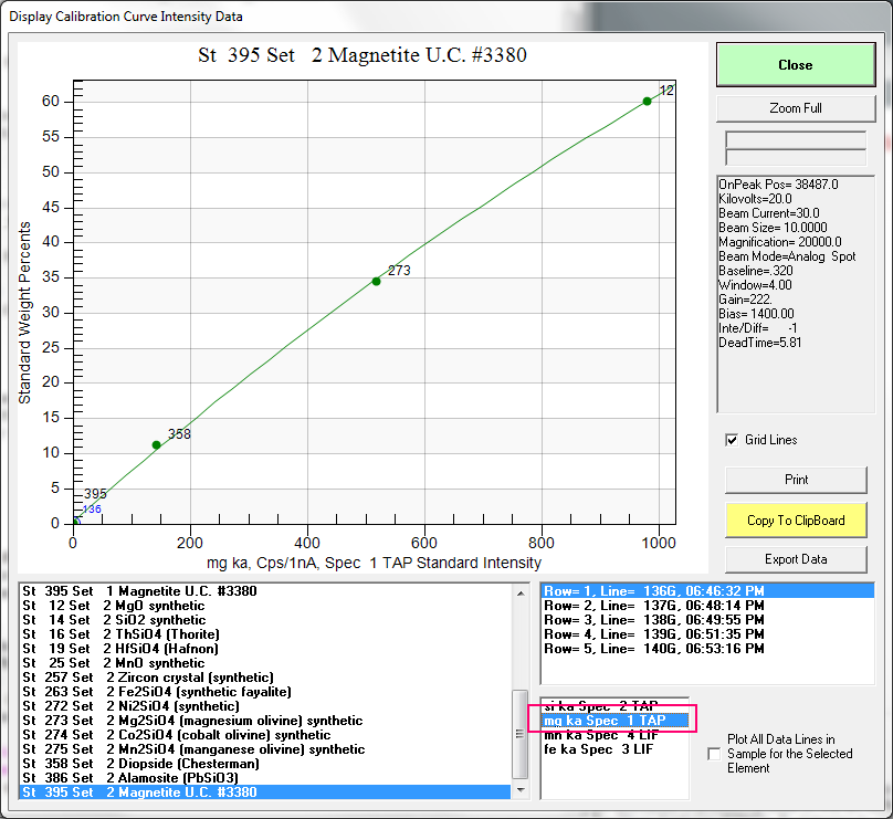
Note that this calibration curve is actually background corrected (see the synthetic zero intensity, zero concentration point), since these standard intensities were acquired using off-peak backgrounds, so the calibration curves are actually based on net intensities, not raw intensities! Which one would generally not have available for quantification, of an x-ray map for example.
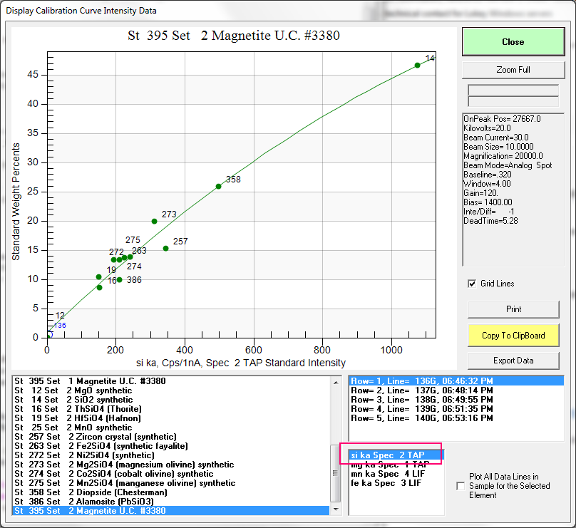
Now from the same silicate run, here is the Si calibration curve:
How does this relate to a quantitative analysis? Well, here is the numerical analysis of a zircon using these Mg and Si calibration curves, and also a few other elements:
ELEM: Si Mg Mn Fe
BGDS: MAN MAN MAN MAN
TIME: 60.00 60.00 60.00 60.00
BEAM: 30.13 30.13 30.13 30.13
ELEM: Si Mg Mn Fe SUM
96 19.071 .480 .045 .058 104.331
97 19.131 .480 .048 .052 104.388
98 19.082 .480 .036 .059 104.334
99 19.065 .478 .046 .055 104.321
100 19.075 .478 .044 .058 104.333
AVER: 19.085 .479 .044 .057 104.342
SDEV: .027 .001 .004 .003 .027
SERR: .012 .001 .002 .001
%RSD: .14 .27 10.17 5.09
PUBL: 15.323 n.a. n.a. n.a. 100.000
%VAR: 24.55 --- --- ---
DIFF: 3.762 --- --- ---
UNCT: 345.22 .86 .61 .71
UNBG: .00 .00 .00 .00
KRAW: 1.0000 1.0000 1.0000 1.0000
PKBG: .00 .00 .00 .00
FIT1: .5391 .4173 -.0963 -.1158
FIT2: .0589 .0726 .2311 .2422
FIT3: -.000015-.000012-.000079-.000093
DEV: 11.7 1.8 .1 .1
Note the large variance for the Si Ka calibration curve and the quite nasty quantification. Bottom line, we cannot rely on calibration curves for x-ray quantification whether they be points or pixels.


 If you are a member, please feel free to add your website URL to your forum profile