Quant Mapping How-To Part 3: Map quantification in CalcImage

[Karsten Goemann]

This is the third part of the 3-part series on how to perform quantitative mapping.

See here for the first part on setup and acquisition of calibration standards in Probe For EPMA:

https://probesoftware.com/smf/index.php?topic=106.0

See here for the second part on map acquisition in ProbeImage:

https://probesoftware.com/smf/index.php?topic=141.0

3. Map quantification in CalcImage

Launch CalcImage. This application is part of the Probe For EPMA package and should reside in the Probe Software/Probe For EPMA folder.

Go to the Project menu and select "Create (new) Project Wizard!":



The software displays step by step instructions how to build the new project:



Click OK. An Open File dialog opens. Find and highlight the Probe for EPMA .MDB database that was created in the Part 1 of the tutorial when setting up the parameters for the map and click "Open":



The software loads the file and displays the instructions for the next step:



Click OK. A window opens displaying all samples in the .MDB file. Select the "quant map setup" sample created in Part 1.  This sample contains all 10 elements to be quantified, as listed on the left hand side of the window. We will combine the two separate Probe Image map acquisitions (5 elements each, same area) into one dataset, so that all major elements are accounted for in the matrix correction. Click OK:



Again, the instructions for the next step are displayed:



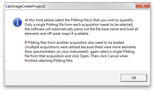
Click OK. Another Open File dialog opens. Select one of the .PRBIMG files for the first map acquision, for example Mg, and click "Open". (Note: do not select one of the electron image files which are VS1, VS2.)



The software will automatically load all x-ray element maps of that acquisition (including optional off-peak images if these were acquired) and create individual Golden Software Surfer .GRD image files. After that's done, the same window opens again. Now select one of the files for the second map acquisition, e.g. Na and click open:



After completion, the same window opens again. As all required files have now been imported, click "Cancel" to stop the importing:



All ten .GRD files are opened and arranged in the main CalcImage window:



A message box is displayed with suggestions for the next steps:



Click OK. Select Project | Specify Quantitative Parameters!:



In this window, first check in the bottom half if the .GRD image files have been assigned correctly to the corresponding elements (including optional off-peak images if these have been acquired). Also, tick the boxes for "Calculate 'Totals' Image" and "Calculate Stoichiometric Oxygen Image". These are useful to assess the quality of the quantification:



The "Calculation Options", "Elements/Cations", "Standard Assignments" and "Specified Concentrations" buttons are similar to Probe For EPMA and can be used to change the corresponding settings. Click for example "Calculation Options" to ensure oxygen is calculated by stoichiometry in the quantification. This is required as the mapped minerals all contain oxygen as the main anion and we did not acquire an oxygen map:



The Analysis | Analysis Options menu can also be used in a way very similar to Probe For EPMA to change global quantification options, for example to use aggregate intensities to combine maps of the same element acquired in parallel on more than one spectrometer.

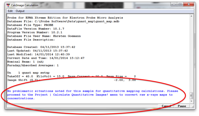
Next, select Project | Output Sample Parameters!:



If no problems with the settings are found, the following message is displayed in the CalcImage Calculation window:



Select Project | Calculate Quantitative Images! to start the map quantification:



A message box appears to double-check everything's ready to go:



Click OK. The quantification starts. Progress and estimated finish time are displayed at the bottom of the window:



After completion, the following message box is displayed:



Click OK. An additional ..._Quant.GRD file has been created in the same directory as the .MDB file for every element and in this case also ..._Oxygen_Quant.GRD and ..._Total.GRD. The project information is stored in the .CIP file. The quantified images are displayed in CalcImage:



To display only the quantified images, select File | Close All Images:



Then select Project | Open Images For Current Project | Open Quant (elemental) Images:





When moving the mouse pointer over the maps, the corresponding X and Y stage coordinates are displayed in the header of the respective image window. The concentration of the element is displayed as the Z value.

In the Processing menu, CalcImage offers further processing capabilities to classify maps, for example to identify different phases and calculate their modal abundances.

For presentation purposes and other operations (such as extracting slices from the maps or calculating average compositions), the maps are exported to Golden Software Surfer. Different output formats are available. For example, to simply export the quantified maps for presentation, select Project | Export the Project Grid Files For Presentation Output | Output Quant Maps To Surfer:



CalcImage then creates a Golden Software .BAS script file:



Click OK. Another message box opens:



Click Yes to run the .BAS file rightaway.  For this to work, Surfer must be installed on the PC and the location must be specified correctly in the Software section of Probewin.INI, e.g.:
SurferAppDirectory="C:\Program Files\Golden Software\Surfer 11"

This opens the applications Scripter and Surfer and performs the operations as specified in the .BAS file. In this case, three Surfer .SRF files and corresponding .JPG image files are created, each containing four maps arranged on one page. The first page as displayed in Surfer is shown below:




This concludes the three part series on how to perform quantitative mapping.

Cheers,

Karsten

[Dan R]

Hi Karsten-
    Is the default .BAS file created for each map for Surfer's Scripter able to be changed? or would I have to manually change each .bas file for each map I make if I wanted to modify the output? Now I typically open up the file in Surfer and make changes if I would like, but I'd like to automate my changes if possible.
-Dan

[Karsten Goemann]

Hi Dan,

John can correct me if I'm wrong, but I don't think there's a direct way for you to change how the .BAS files are created by CalcImage. This would require adding further output options into CalcImage according to your specifications.

But you could modify the .BAS scripts created by CalcImage before running them, or make your own to automate specific tasks. You could run those instead of the ones created by CalcImage, or for example use the .SRF files created by the existing CalcImage output routines and just modify them further with your own .BAS scripts.

I haven't done much scripting in Surfer myself, but here's for example a thread started by John about modifying the .BAS scripts:
http://probesoftware.com/smf/index.php?topic=55.0

Cheers,

Karsten

[John Donovan]

This is an great example of why these scripts are so powerful. They are easily modified as Karsten points out above.

So, yes, occasionally I will update the "core" scripts for the purposes of adding a feature, but at the moment these scripts are pretty complete (exception: the polygon scripts are not completely finished). In any case, if you "customize" these scripts for your own lab, to preserve your modifications, it is a good idea to make copies of your modified scripts and overwrite the default scripts after each PFE software update.

Here is a listing of the "core" scripts that are used by CalcImage to create new output:

SLICEXY.BAS     Profile "slicing" of map data using N "anchor points"
http://probesoftware.com/smf/index.php?topic=41.msg541#msg541

STRIPXY1.BAS   Pixel averaging via user defined "strips" (square maps)
STRIPXY2.BAS   Pixel averaging via user defined "strips" (tall maps)
STRIPXY3.BAS   Pixel averaging via user defined "strips" (wide maps)
http://probesoftware.com/smf/index.php?topic=41.msg897;topicseen#msg897

POLYXY.BAS      Pixel averaging via user defined polygon
http://probesoftware.com/smf/index.php?topic=41.msg543#msg543

I will eventually be adding a traverse script for PFE for creating easy to modify presentation quality plots, but the scripts listed above are the ones used for x-ray mapping output.

[John Donovan]

    Is the default .BAS file created for each map for Surfer's Scripter able to be changed? or would I have to manually change each .bas file for each map I make if I wanted to modify the output? Now I typically open up the file in Surfer and make changes if I would like, but I'd like to automate my changes if possible.

To create customized scripts for output that will not get overwritten when you update PFE, please see this post:

http://probesoftware.com/smf/index.php?topic=305.msg1560#msg1560

[John Donovan]

Ben Buse recently contacted us because he was trying to create a new CalcImage quant mapping project with (three) multiple spectrometer passes (for quantifying more elements than spectrometers), but when he tried to load the GRD files automatically using the New Project Wizard as described in the first post in this topic, he got a warning that at least one of the x-ray maps being loaded did not match the electron beam energy of the Probe for EPMA sample basis as seen here:



This is because the New Project Wizard assumes that only a single KeV was utilized in the acquisition of the x-ray maps for quantification. But he acquired the spectrometer passes using different keVs!  However, the sample basis in Probe for EPMA was a so called "combined condition" samples, so CalcImage should have allowed it.

We will fix this issue in a future version, but if you do want to acquire multiple spectrometer passes each at different electron beam energies, as Ben pointed out, one can simply use the manual project  menus in CalcImage as seen here:



That is, first start by creating a new project, and then using each of the Project | Add... menus specify the MDB file, the sample basis, and each of the x-ray map files you want to load into the project.

Then just use the Project | Specify Quantitative Parameters menu as usual.