Author Topic: Statistics in Quantitative X-ray Maps  (Read 1318 times)

Ben Buse

  • Professor
  • ****
  • Posts: 488
Statistics in Quantitative X-ray Maps
« on: April 21, 2022, 08:31:44 AM »
Regarding 'A new EPMA method for fast trace element analysis in simple matrices'

''The precision errors of the MAN background calibration are smaller than direct background measurement'

Is this implemented in the calculation of the counting time errors (analytical sensitivity) for the maps when using MAN?

Thanks

Ben
« Last Edit: April 22, 2022, 08:53:33 AM by John Donovan »

Probeman

  • Emeritus
  • *****
  • Posts: 2836
  • Never sleeps...
    • John Donovan
Re: Statistics in Quantitative X-ray Maps
« Reply #1 on: April 21, 2022, 12:13:34 PM »
Hi Ben,

Great question.

So do we apply the improved MAN statistics to the analytical sensitivity calculation?  Assuming you are speaking of the single point/single pixel calculations, the simple answer is no, we only apply the MAN statistics to the detection limit calculation.  For the benefit of others, I'm going to detail these considerations, though I'm sure you already know most of this since you've read the paper, which is here for others if interested:

https://pubs.geoscienceworld.org/msa/ammin/article-abstract/101/8/1839/264218/A-new-EPMA-method-for-fast-trace-element-analysis

The reason for this decision (and we are willing to discuss the pros and cons), is that the analytical sensitivity calculation is dominated by the peak to background ratios, while the detection limit calculation is dominated by the variance of the background statistics. So in the analytical sensitivity calculation, as the P/B approaches 1, the square root doesn't change, so I think MAN statistics would have little effect on the analytical sensitivity calculation.

This can be seen is the single point/pixel expressions for both calculations:


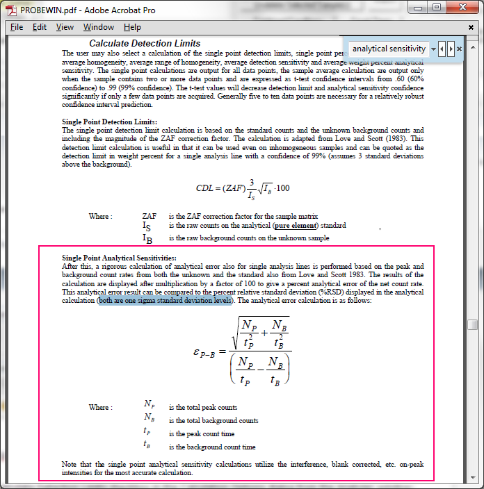
In fact we don't even display analytical sensitivity calculations for concentrations under 1 wt%.  When estimating sensitivity, the detection limit is a more accurate description of trace element sensitivity.

The improved statistics for the MAN background method, results in approximately the same (average) background intensity, but the variance is much lower.  So the actual background intensity is roughly the same. What the Scott and Love analytical sensitivity calculation assumes is Gaussian statistics for the background measurement, by taking the square root of the background. The same assumption is made for the detection limit calculation.

And this assumption is correct when the background is measured using the off-peak method, because it is a direct measurement of the continuum intensities.  However, the MAN background is instead a regression of the average of many continuum intensities, in standards where the element is not present. So the variance is dependent on two things, first the variance of the *major* elements. Because that variance in the average Z affects the variance of the MAN intensity. And second the magnitude of the average Z, because the intensity of the background usually increases with increasing average Z.

But remember, the MAN regression is not re-measured for each point or pixel. Instead it is generally acquired once per run, and calculated for each point/pixel based on the iterated average Z.  If the average Z does not change, then the MAN background intensity does not change for all points/pixels.

In fact the background variance is zero if the average Z is exactly the same. Imagine an MAN calibration curve where the major elements are either specified or by difference, so for example trace Ti in quartz, where Ti is measured and SiO2 is specified or by difference.  Whether the SiO2 is specified or by difference, the average atomic number of this material is dominated by the SiO2 concentrations, while the variation of trace Ti will only affect the average Z in the 4th or 5th decimal place.

In other words the MAN background variance is often very close to zero, but depends on whether the matrix (major) elements are measured, or specified by  composition or by difference. Since the variances of the peak and background are added in quadrature, the limiting factor of the background variance is the variance of the on-peak measurement. This basically results in an improvement in the MAN detection limit of around 30 to 40%.

So, as mentioned above, we only apply the improved MAN statistics to the detection limit calculation. If you have any ideas on why it would be useful to apply the MAN statistics to the analytical sensitivity calculation I would like to hear them, but remember, we don't display analytical sensitivity for concentrations less than 1 wt%.

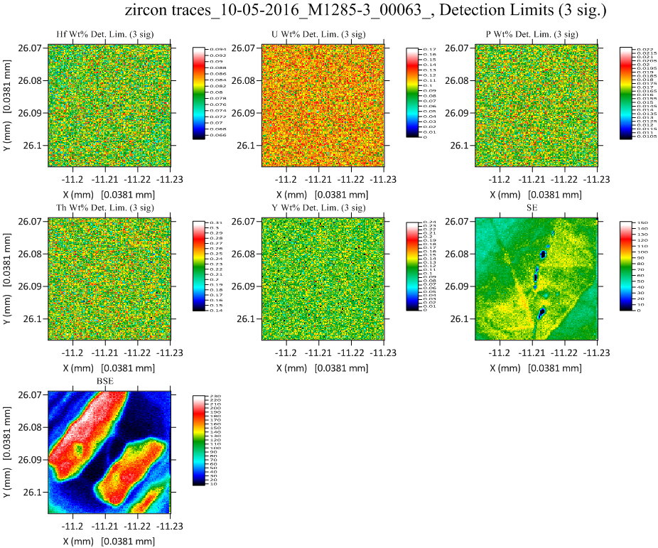
Figure 13 in the MAN paper shows the detection limit improvement for MAN backgrounds on a homogeneous synthetic zircon, but a better example might have been using a natural zircon as seen in these images below.  As with figure 13, off-peak maps were acquired for the zircon, and utilized in the off-peak quantification, but not utilized in the MAN quantification (normally resulting in an acquisition time half that for off-peak quantification). Here are the off-peak per pixel detection limits:


And here are the MAN per pixel detection limits:


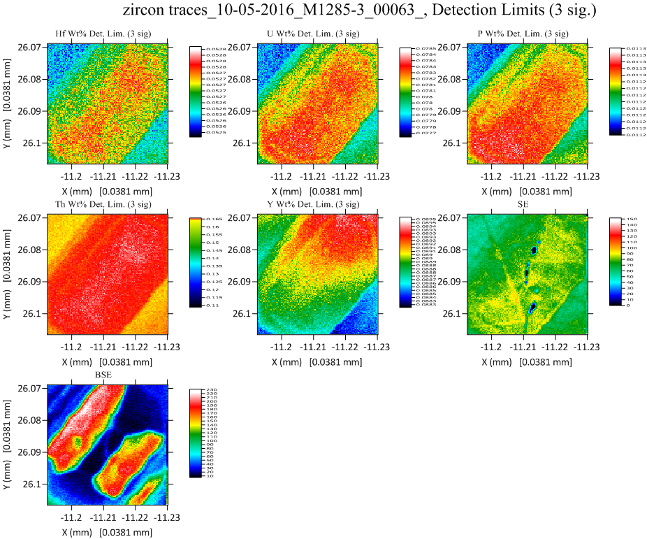
If you can read the Z labels (just click on the images to make them full size), you can see the off-peak detection limit statistics are significantly worse than the MAN statistics, and the MAN detection limits actually show slightly higher detection limits as the concentration of Hf (a high Z element) increases in the core of the zircon. This is as mentioned above due to the slope of the MAN curve (usually) increasing with increasing average atomic number. Here ZrSiO4 was specified by difference from 100%, so the MAN background variance was very close to zero.

Hope that helps.
« Last Edit: April 22, 2022, 08:53:41 AM by John Donovan »
The only stupid question is the one not asked!

Ben Buse

  • Professor
  • ****
  • Posts: 488
Re: Statistics in Quantitative X-ray Maps
« Reply #2 on: April 22, 2022, 08:32:28 AM »
Hi John,

Thank you for that detailed explanation of what you do and why.

A further clarification for 'extract polygon areas and/or perform pixel filtering', for the map or a box or a polygon you can extract average composition and std devs or std errs.

Here is this the standard deviation of the average compostion within the box. And for std err this is the standard error on the std dev.

Sorry that doesn't make much sense - what I'm saying is these values are based on the measurements in question and do not use the counting statistic formulas.

Why I'm interested is frequently we do trace element mapping, filter out bad data in calcimage and then extract wide lines using imagej, the question is then on that line profile what is the error bar?

Just come across an interesting plugin for imagej https://imagej.nih.gov/ij/macros/PlotProfileWithSD.txt

Ben
« Last Edit: April 22, 2022, 08:53:57 AM by John Donovan »

John Donovan

  • Administrator
  • Emeritus
  • *****
  • Posts: 3275
  • Other duties as assigned...
    • Probe Software
Re: Statistics in Quantitative X-ray Maps
« Reply #3 on: April 22, 2022, 09:00:16 AM »
Hi Ben,
I'm not sure I understand exactly what you are getting at. 

But let me start by saying that the standard deviation is not the ideal statistic for averaging pixels because it doesn't improve with the number of pixels being averaged. In fact I think it was you (wasn't it?) that asked for the standard error calculation since that improves with the number of pixels being averaged.

Quote
Why I'm interested is frequently we do trace element mapping, filter out bad data in calcimage and then extract wide lines using imagej, the question is then on that line profile what is the error bar?

If you are modifying the number of pixels in an external program then of course the standard error will change and would need to be re-calculated.

What I do to "filter out bad data" is to use the polygon feature to avoid pits and cracks as described here:

https://probesoftware.com/smf/index.php?topic=877.msg5584#msg5584
John J. Donovan, Pres. 
(541) 343-3400

"Not Absolutely Certain, Yet Reliable"

Probeman

  • Emeritus
  • *****
  • Posts: 2836
  • Never sleeps...
    • John Donovan
Re: Statistics in Quantitative X-ray Maps
« Reply #4 on: April 22, 2022, 09:15:03 AM »
But let me start by saying that the standard deviation is not the ideal statistic for averaging pixels because it doesn't improve with the number of pixels being averaged.

From what I understand this is because the standard deviation is the variance for each single data point (or pixel), while the standard error is the variance for the average of all points (or pixels).

Therefore when we plot a single point (or pixel), we should utilize the standard deviation, but when we plot the average of the points (or pixels) we should utilize the standard error.  Tip: look up standard deviation and standard error in the Probe for EPMA reference manual glossary and this will make sense.

As to why we usually see the average and the standard deviation quoted together, I once asked a statistician this question and they responded: good question, no idea...
The only stupid question is the one not asked!

Ben Buse

  • Professor
  • ****
  • Posts: 488
Re: Statistics in Quantitative X-ray Maps
« Reply #5 on: April 25, 2022, 06:13:31 AM »
Thanks and sorry,

Was just thinking aloud, about the best why to determine the error for a group of pixels in an x-ray map at trace element concentration.

Either put it through the counting statistics formula

Or determine standard deviation and from it calculate standard error.

Then its which is easiest to do for the presented results - in this case a wide line

« Last Edit: April 25, 2022, 06:37:39 AM by Ben Buse »

Ben Buse

  • Professor
  • ****
  • Posts: 488
Re: Statistics in Quantitative X-ray Maps
« Reply #6 on: April 25, 2022, 08:35:50 AM »
So modifying

https://imagej.nih.gov/ij/macros/PlotProfileWithSD.txt

and

https://imagej.nih.gov/ij/macros/StackProfilePlot.txt which I'd previously modified to work with multiple channels rather than slices

Gives a macro that plots a line with an error bar which signifies either the standard deviation or the standard error, of the range of data constituting the line

i.e. its a wide line (data averaged either side of the central line) - with standard deviation or standard error shown

Great  :)

So trace element quant maps with holes excluded through filtering in calcimage, then into imagej, plot width averaged line profile, and assign error  :)
« Last Edit: April 25, 2022, 08:40:15 AM by Ben Buse »

John Donovan

  • Administrator
  • Emeritus
  • *****
  • Posts: 3275
  • Other duties as assigned...
    • Probe Software
Re: Statistics in Quantitative X-ray Maps
« Reply #7 on: April 25, 2022, 09:39:08 AM »
Hi Ben,
This looks interesting. Thanks for showing us these macros. Also, please feel free to show us an example of the output from this macro.

These line profiles with statistics can also (sort of) be accomplished using the line profile feature in CalcImage, if one selects the standard error output option, and selects the export to file checkbox as shown here:


But it outputs a separate file for each area, which looks like this in Excel:


This all reminds me of this conversation from three years ago:

https://probesoftware.com/smf/index.php?topic=1144.msg8000#msg8000

In the case of these traces in zircon, it would look like this:


And of course now, I realize that one can then export the data from this plot using the Export Data button...

OK, but I just looked at this output file and the concentrations are there but the deviations are all zero, so let me take a look and see if I can fix that today.
John J. Donovan, Pres. 
(541) 343-3400

"Not Absolutely Certain, Yet Reliable"

John Donovan

  • Administrator
  • Emeritus
  • *****
  • Posts: 3275
  • Other duties as assigned...
    • Probe Software
Re: Statistics in Quantitative X-ray Maps
« Reply #8 on: April 25, 2022, 11:38:33 AM »
Ha!   I thought we had a bug but I was wrong!     8)
 
I had just quickly glanced at the last few columns of data which was for the O, Si and Zr columns, but since I specified ZrSiO4 by difference, and didn't map them, those columns *would* be zero!

Doh!

In fact, the averages and standard deviations or standard errors are correctly exported as shown here:


So if one would like to get a wide "strip" of averages for trace elements from a quant map simply use the Export Data button as seen here:


That will create a tab delimited ASCII (text) file which can be easily opened in Excel or any graphing program.

The size of the extraction square can be adjusted to get a nice fit of averaging versus spatial resolution as seen here:


Remember, these calculated error bars are 1 sigma statistics, so you might want to multiply them by 3 to get 99% statistics...
« Last Edit: April 25, 2022, 11:46:04 AM by John Donovan »
John J. Donovan, Pres. 
(541) 343-3400

"Not Absolutely Certain, Yet Reliable"

JonF

  • Professor
  • ****
  • Posts: 149
Re: Statistics in Quantitative X-ray Maps
« Reply #9 on: April 27, 2022, 02:49:39 AM »
I've been telling our users to do the line profiles the same way Ben suggests.

My rationale is that in ImageJ, I think the "wide" line profile averages pixels perpendicular to the orientation of the profile line, whereas CalcImage averages pixels in a square around the pixel selected.
For CalcImage, this results in the exported dataset being averaged along the direction of the profile line, causing what would be a sharp boundary to become sigmoidal.

This is a gut feeling though - I've not actually got round to testing ImageJ to make sure it is doing what I think it is!

Ben Buse

  • Professor
  • ****
  • Posts: 488
Re: Statistics in Quantitative X-ray Maps
« Reply #10 on: April 27, 2022, 03:41:35 AM »
So here's an example. Data can be filtered in calcimage first to remove holes etc.

1. Create stack of multiple channels - as posted elsewhere https://probesoftware.com/smf/index.php?topic=799.msg9557#msg9557.


2. Rotate stack so wide line is horizontal.


3. Draw profile box


4. Run macro to plot profile with error bars of standard deviation


5. Run macro to plot profile with error bars of standard error


Left to right is plot. Scale currently in pixels not microns  ???
« Last Edit: April 27, 2022, 03:56:19 AM by Ben Buse »

Ben Buse

  • Professor
  • ****
  • Posts: 488
Re: Statistics in Quantitative X-ray Maps
« Reply #11 on: April 27, 2022, 04:29:30 AM »
Updated macro scaled


Here's the script for standard error

Code: [Select]
// modified from https://imagej.nih.gov/ij/macros/StackProfilePlot.txt
// StackProfilePlot
// This macro generates profile plots of all the images
// in a stack and stores then in another stack.

macro "Stack profile Plot" {
    ymin = 0;
    ymax = 255;
    saveSettings();
    Stack.getDimensions(width,height,channels,slices,frames);
    getVoxelSize(vwidth,vheight,vdepth,vunit);
    if (channels==1)
      exit("Channel Stack required");
// remove comments if wish to fix min and max y scale for all channels
//    run("Profile Plot Options...",
//      "width=400 height=200 minimum="+ymin+" maximum="+ymax+" fixed");
    setBatchMode(true);
    stack1 = getImageID;
    stack2 = 0;
    c = channels+1;
    for (l=1; l<c; l++) {
        showProgress(l, c);
        selectImage(stack1);
        Stack.setChannel(l);
        errorBarScale = 1;
        if (selectionType!=0)
            exit("Rectangular selection required");
        getSelectionBounds(xbase, ybase, width, height);
        profile = newArray(width);
        sd = newArray(width);
        xprofile = newArray(width);
areaprofile = newArray(width);
        n = height;
//        print(n);
//        print(width);
//        print(width*vwidth);
        for (x=xbase; x<xbase+width; x++) {
            makeRectangle(x, ybase, 1, height);
            getStatistics(area, mean, min, max, std);
            profile[x-xbase] = mean;
            xprofile[x-xbase] = x-xbase;
            sd[x-xbase] = std;
            areaprofile[x-xbase] = area/vwidth/vwidth;
        }
        makeRectangle(xbase, ybase, width, height);
        run("Clear Results");
        for (i=0; i<width; i++) {
            setResult("Mean", i, profile[i]);
            setResult("Distance", i, xprofile[i]);
            setResult("SD", i, sd[i]);
            setResult("NumberOfPixels", i, areaprofile[i]);
            sd[i] /= sqrt(areaprofile[i]);
            xprofile[i] *=vwidth;
        }
        updateResults;
        if (l==1) {
        Plot.create("Profile Plot"+l, "X"+vunit, "Wt. %", xprofile, profile);
        Plot.add("error bars", xprofile, sd);
        } else {
        Plot.add("line", xprofile, profile);
        Plot.add("error bars", xprofile, sd);
        }
//        Table.rename("Results", "Results-"+l);
    }
    Stack.setChannel(1);
    setBatchMode(false);
    restoreSettings();
}
« Last Edit: April 27, 2022, 05:00:01 AM by Ben Buse »

JonF

  • Professor
  • ****
  • Posts: 149
Re: Statistics in Quantitative X-ray Maps
« Reply #12 on: April 27, 2022, 04:40:01 AM »
Rather than rotating the image and drawing a box, could you use the straight line tool to draw a profile line, then double click on the straight line tool icon and specify the line width?

I don't know if drawing the box was a specific requirement of the macro, but could save you some time being able to arbitrarily draw lines rather than rotating the image stack.


Ben Buse

  • Professor
  • ****
  • Posts: 488
Re: Statistics in Quantitative X-ray Maps
« Reply #13 on: April 27, 2022, 05:02:44 AM »
Hi Jon,

Yes that's what I've previously done to create stack plots, see attached marcos in post https://probesoftware.com/smf/index.php?topic=799.msg9557#msg9557 however no error bar

The difference here is to create the error bar - and adapting someone's macro (https://imagej.nih.gov/ij/macros/PlotProfileWithSD.txt) - the line is then made up of rectangles for which the standard deviation can be returned, from which the standard error can be calculated

Ben
« Last Edit: April 27, 2022, 05:11:06 AM by Ben Buse »

JonF

  • Professor
  • ****
  • Posts: 149
Re: Statistics in Quantitative X-ray Maps
« Reply #14 on: April 27, 2022, 07:10:44 AM »
I see what you mean. It's quite annoying that the Profile Plot knows enough to average the data, but not to save all the pixels that it uses in the averaging...

The code for ProfilePlot is on github: https://github.com/imagej/ImageJ/blob/master/ij/gui/ProfilePlot.java

I suspect the information you would need would be in the getWideLineProfile() function. 
Confusingly, it looks like "height" might be what we're calling line "width", with the "width" actually being the line length. Argh.

I think it's drawing a series of parallel lines, starting at y=0 and adding all the pixel values along the profile length to profile(i). It then goes to y=1 and adds the new pixel values to the already collected values for each position along the profile line, and so on until y = height ("line width?"). It then divides profile(i) by the height and then spits out the array "profile". 
What we need to do is add another array in there to store all the individual pixels in profile(y,i) and then get that spat out, too. Or calculate the SD as part of the script and dump that instead.   

« Last Edit: April 27, 2022, 07:20:47 AM by JonF »