New method for calibration of dead times (and picoammeter)

[Brian Joy]

Your uncorrected data are difficult to interpret in part because both the primary and secondary standards require large, non-linear dead time corrections that lead to a roughly linear appearance of the uncorrected plot of k-ratio versus current.  You also haven’t presented peak searches or wavelength scans so that peak shapes can be compared at increasing count rates.

This is what you keep saying but I really don't think you have thought this through.   There is nothing non-linear about the expanded dead time correction. The dead time expression (all of them) are merely a logical mathematical description of the probability of two photons entering the detector within a certain period of time.

Linear:  N'/N = 1 – N’τ (slope = -τ)
Non-linear:  N'/N = 1 – (N’τ + N’²(τ²/2))

[Probeman]

Your uncorrected data are difficult to interpret in part because both the primary and secondary standards require large, non-linear dead time corrections that lead to a roughly linear appearance of the uncorrected plot of k-ratio versus current.  You also haven’t presented peak searches or wavelength scans so that peak shapes can be compared at increasing count rates.

This is what you keep saying but I really don't think you have thought this through.   There is nothing non-linear about the expanded dead time correction. The dead time expression (all of them) are merely a logical mathematical description of the probability of two photons entering the detector within a certain period of time.

Linear:  N/N’ = 1 – N’τ (slope = -τ)
Non-linear:  N/N’ = 1 – (N’τ + N’²(τ²/2))

Now you're just arguing semantics. Yes, the expanded expression is not a straight line the way you're plotting it here (nice plot by the way!), but why should it be? It's a probability series that produces a linear response in the k-ratios. Hence "constant" k-ratios.   

It's the additional terms of the Taylor expansion series which is why it works at high count rates. Whereas the single term expression fails miserably, as you have already acknowledged.

And as your plot nicely demonstrates, and I have noted previously, there is little to no difference at low count rates, and hence no "non-linearities" that you seem to be so concerned with. This is good news for everyone because the more precise dead time expressions can be utilized under all beam current conditions.

Think about it: plotting these expanded expressions on a probability scale would produce a line that approaches a straight line. That's the point about "linear" that I've been trying to make clear.

And if you plot up the six term dead time expression you will find that it approaches the actual probability of a dead time event more accurately at even higher count rates. As demonstrated by the constant k-ratio data from both JEOL and Cameca instruments in this topic.

[Probeman]

Here's something interesting that I just noticed.

When I looked at the dead times Anette had in her SCALERS.DAT file, and the dead times after she optimized them with her Te, Se and Ti k-ratio data, there is an obvious shift from higher to lower dead times constants:

Ti Ka dead times, JEOL iHP200F, UBC, von der Handt, 07/01/2022
Sp1     Sp2    Sp3     Sp4     Sp5
PETJ    LIFL    PETL   TAPL    LIFL
1.26   1.26    1.27    1.1     1.25          (usec) optimized using constant k-ratio method
1.52   1.36    1.32    1.69    1.36         (usec) JEOL engineer using traditonal method

I suspect that the reason she found smaller dead time constants using the constant k-ratio method is because she has an instrument that produces quite high count rates, so when the JEOL engineer tried to compensate for those higher count rate (using the traditional dead time expression), he had to increase the apparent dead time constants to get something that looked reasonable. And the reason is of course that the traditional dead time expression just doesn't cut it at count rates attained at even moderate beam currents on these new instruments.

In fact I found exactly the same thing on my SX100. Using the traditional single term expression I found I was having to increase my dead time constants to around 4 usec!  That was when I decided to try the existing "high" precision (two term) expression from Willis (1993).  And that helped but it still was showing problems at count rates exceeding 100K cps.

So that is when John Fournelle and I came up with the expanded dead time expression with 6 terms. Once that was implemented everything fell nicely into place and now we can get consistently accurate k-ratios at count rates up to 500K cps or so with dead time constants at or even under 3 usec!  Of course above that 500 K cps count rate we start seeing the WDS detector showing a little of the "paralyzing" behavior discussed earlier. 

I'm hoping that Mike Jercinovic will perform some of these constant k-ratio measurements on his VLPET (very large) Bragg crystals on his UltraChron instrument and see what his count rates are at 200 nA!   

It's certainly worth considering how much of a benefit this new expression is for new EPMA instruments with large area crystals. For example, on Anette's PETL Bragg crystals she is seeing count rates on Ti Ka of around 2800 cps/nA. So at 10 nA she's getting 28K cps and at 30 nA she's getting around 84K cps!

That means that using the traditional dead time expression she's already seeing accuracy issues at 30 nA!  And wouldn't we all like to go to beam currents of more than 30 nA and still be able to perform accurate quantitative analyses?

 

[Probeman]

Brian Joy's plots of the traditional and Willis (1993) (two term) dead time expressions are really cool, so I added the six term expanded dead time expression to this plot. 

First I wrote code to calculate the dead time corrections for all of the Taylor series expressions from the traditional (single term) to the six term expression that we call the "super high" precision expression. It's extremely simple to generate the Taylor series to as many terms as one wants, as seen here:

Code: [Select]

' For each of the number of Taylor expansion terms
For j& = 0 To 5

temp2# = 0#
For i& = 2 To j& + 1
temp2# = temp2# + cps& ^ i& * (dtime! ^ i&) / i&
Next i&
temp# = 1# - (cps& * dtime! + temp2#)
If temp# <> 0# Then corrcps! = cps& / temp#

' Add to output string observed cps divided by corrected (true)
astring$ = astring$ & Format$(CSng(cps& / corrcps!), a80$) & vbTab
Next j&

The output from this calculation is seen here:



The column headings indicates the number of Taylor probability terms in each of the columns (1 = the traditional single term expression). This code is embedded in the TestEDS app under the Output menu but the modified app has not yet been released by Probe Software as yet!

Plotting up the traditional, Willis and six term expressions we get this plot:



The 3, 4 and 5 term expressions plot pretty much on top of each other since this plot only goes up to 200K cps, so they are not shown, but you can see the values in the text output.  On a JEOL instrument with ~1.5 usec dead times, up to about 50K to 80K cps, the traditional expression does a pretty good job, but above that the Willis (1993) expression does better, and above 160K cps we need the six term expression for best accuracy.

As we saw from our constant k-ratio data plots, the six term expression really gets going at 200K cps and higher.

[Probeman]

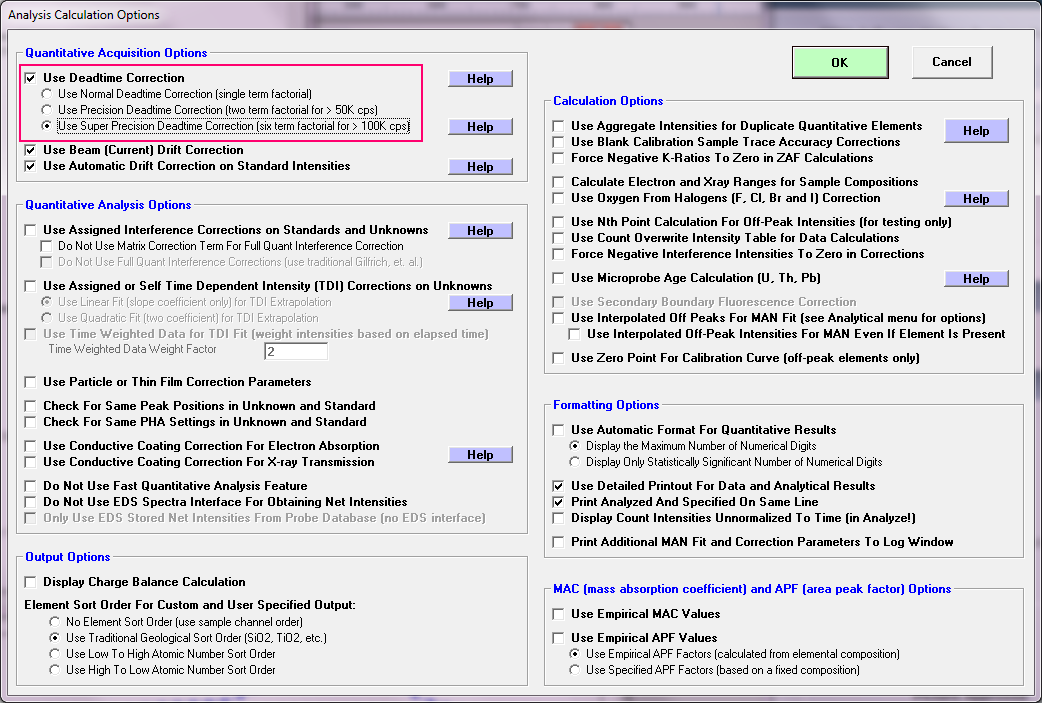
We modified the TestEDS app a bit to only display results for only the traditional (single term), Willis (two term) and the new six term expression dead time expressions. And we increased the observed count rates to 300K cps and also added output of the predicted (dead time corrected) count rates as seen here:



Note that this version of TestEDS.exe is available in the latest release of Probe for EPMA (using the Help menu).

Now if instead of plotting the ratio of the observed to predicted count rates on the Y axis, we instead plot the predicted count rates themselves, we can see this plot:



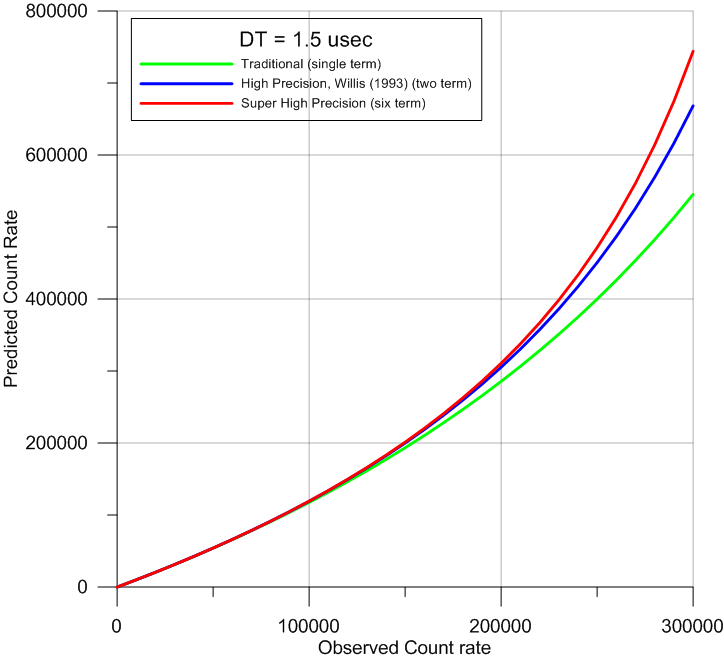
Note that unlike the ratio plot, all three of the dead time correction expressions show curved lines.  This is what I meant when I stated earlier that it depends on how the data is plotted.

Note also that at true (corrected) count rates around 400 to 500K cps we are seeing differences in the predicted intensities between the traditional expression and the new six term expression of around 10 to 20%!

To test the six term expression we might for example measure our primary Ti metal standard at say 30 nA, and then a number of secondary standards (TiO2 in this case) at different beam currents, and then plot the k-ratios for a number of spectrometers first using the traditional dead time correction expression:



Note spectrometer 3 (green symbols) using a PETL crystal.  Next we plot the same data, but this time using the new six term dead time correction expression:



The low count rate spectrometers are unaffected, but the high intensities from the large area Bragg crystal benefit significantly in accuracy. 

I can imagine a scenario where one is measuring one or two major elements and 3 or 4 minor or trace elements, using 5 spectrometers. The analyst measures all the primary standards at moderate beam currents, but in order to get decent sensitivity on the minor/trace elements the analyst selects a higher beam current for the unknowns. 

Of course one can use two different beam conditions for each set of elements, but that would take considerably longer.  Now we can do our major and minor elements together using higher beam currents and not lose accuracy.   

I've always mentioned that for trace elements, background accuracy is more important than matrix corrections, but that's only because our matrix corrections are usually accurate to 2% relative or so.  Now that we know that we can see 10 or 20% relative errors in our dead time corrections at high beam currents, I'm going to modify that now and say, that the dead time corrections might be another important source of error for trace and minor elements if one is using the traditional (single term) dead time expression at high beam currents.

The good news is that the six term expression has essentially no effect at low beam currents, so simply select the "super high" precision expression as your default and you're good to go!



Test it for yourself using the constant k-ratio method and feel free to share your results here. 

[Brian Joy]

First I wrote code to calculate the dead time corrections for all of the Taylor series expressions from the traditional (single term) to the six term expression that we call the "super high" precision expression. It's extremely simple to generate the Taylor series to as many terms as one wants, as seen here:

Code: [Select]

' For each of the number of Taylor expansion terms
For j& = 0 To 5

temp2# = 0#
For i& = 2 To j& + 1
temp2# = temp2# + cps& ^ i& * (dtime! ^ i&) / i&
Next i&
temp# = 1# - (cps& * dtime! + temp2#)
If temp# <> 0# Then corrcps! = cps& / temp#

' Add to output string observed cps divided by corrected (true)
astring$ = astring$ & Format$(CSng(cps& / corrcps!), a80$) & vbTab
Next j&


For a given function, f(x), the Taylor series generated by f(x) at x = a is typically written as

f(a) + (x-a) f’(a) + (x-a)²f’’(a)/2! + … + (x-a)ⁿf(n)(a)/n! +…

If a = 0, it is often called the Maclaurin series.  For example, the Maclaurin series for f(x) = exp(-x) looks like this:

exp(-x) = 1 – x + x²/2 – x³/6 + x⁴/24 – x⁵/120 + x⁶/720 + … + (-x)ⁿf⁽ⁿ⁾(0)/n! +…

Just for the sake of absolute clarity, could you identify the function, N(N’), that you’re differentiating to produce the Taylor or Maclaurin polynomial (where N’ is the measured count rate and N is the corrected count rate)?  I’m specifically using the term “polynomial” because the series, which is infinite, has been truncated.

The function, N(N’), presented by J. Willis is

N = N’/(1 – (τN’+τ²N’²/2))

where τ is a constant.  How exactly does the polynomial generated from the identified function relate to the expression presented by Willis?

[Probeman]

I've been writing up this constant k-ratio method and the new dead time expressions up with several of our colleagues (Aurelien Moy, Zack Gainsforth, John Fournelle, Mike Jercinovic and Anette von der Handt) and hope to have a manuscript ready soon.  So if it seems I've been holding my cards close to my chest, that's the reason why!   

Using your notation the expanded expression is:



or


 
I've been calling it a Taylor series, because it is mentioned in the Taylor series Wiki page, but yes, the Maclaurin expression is an exponential version of the Taylor series which is what we are approximating:

https://en.wikipedia.org/wiki/Taylor_series

We are actually using the logarithmic equation now as it works at even higher input count rates (4000K cps anyone?).

Your comments have been very helpful in getting me to think through these issues, and we will be sure to acknowledge this in the final manuscript.

I'll share one plot from the manuscript which pretty much sums things up:



Note that the Y axis (predicted count rate) is in *millions* of cps!

[Probeman]

Here's another way to think of these dead time expressions that Zack, Aurelien and I have come up with:

The traditional (single term) dead time correction expression does describe the probability of a single photon being coincident with another photon, but it doesn't handle the case where two photons are coincident with another photon.
 
That's what the Willis (two term) expression does.

The expanded expression handles three photons coincident with another photon, etc., etc.   The log expression will handle this even more accurately.  Of course at some point the detector physics comes into play when the bias voltage doesn't have time to clear the ionization from the previous event.  Then the detector starts showing paralyzing behavior as has been pointed out.

What amazing is that we are seeing these multiple coincident photon events even at relatively moderate count rates and reasonable dead times, e.g., >100K cps and 1.5 usec. 

But it makes some sense because if you think about it, a 1.5 usec dead time corresponds to a count rate of 1/1.5 usec or about 600K cps assuming no coincident events.

[Brian Joy]

Using your notation the expanded expression is:


 
I've been calling it a Taylor series, because it is mentioned in the Taylor series Wiki page, but yes, the Maclaurin expression is an exponential version of the Taylor series which is what we are approximating:

https://en.wikipedia.org/wiki/Taylor_series

We are actually using the logarithmic equation now as it works at even higher input count rates (4000K cps anyone?).

A human-readable equation is nice.  Picking through someone else’s code is never fun.

This is the Taylor series generated by ln(x) at x = a (for a > 0):

ln(x) = ln(a) + (1/a)(x-a) – (1/a²)(x-a)²/2 + (1/a³)(x-a)³/3 – (1/a⁴)(x-a)⁴/4 + … + (-a)^n-1(n-1)!(x-a)ⁿ/n! + …

Note that the sign alternates from one term to the next.  A Maclaurin series cannot be generated because ln(0) is undefined.

I don’t see how this Taylor series relates to the equation you’ve written.  I also don’t see how it’s physically tenable, as it can’t be evaluated at N’ = N = 0 (but your equation can be).  When working with k-ratios, N’ = N = 0 is the point at which the true k-ratio for given effective takeoff angle is found.

I'm confused, but maybe I'm just being dense.

[Probeman]

You're welcome!

You seem to be focusing on nomenclature. If you need to call it something, call it a Maclaurin-like form of the series. I don't see a problem with a zero count rate. It the count rate is zero, we just return a zero for the corrected count rate.

I'm not confused, probably I'm just being dense.   

[Brian Joy]

You're welcome!

You seem to be focusing on nomenclature. If you need to call it something, call it a Maclaurin-like form of the series. I don't see a problem with a zero count rate. It the count rate is zero, we just return a zero for the corrected count rate.

I'm not confused, probably I'm just being dense.   

It's not an issue of nomenclature.  The Taylor series generated by ln(x) blows up when x = 0.

[Probeman]

You're welcome!

You seem to be focusing on nomenclature. If you need to call it something, call it a Maclaurin-like form of the series. I don't see a problem with a zero count rate. It the count rate is zero, we just return a zero for the corrected count rate.

I'm not confused, probably I'm just being dense.   

It's not an issue of nomenclature.  The Taylor series generated by ln(x) blows up when x = 0.

As you pointed out, it's not exactly a Taylor series.

I could make a joke here about "natural" numbers, but instead I'll ask: what is the meaning of zero incident photons?

[Brian Joy]

You're welcome!

You seem to be focusing on nomenclature. If you need to call it something, call it a Maclaurin-like form of the series. I don't see a problem with a zero count rate. It the count rate is zero, we just return a zero for the corrected count rate.

I'm not confused, probably I'm just being dense.   

It's not an issue of nomenclature.  The Taylor series generated by ln(x) blows up when x = 0.

As you pointed out, it's not exactly a Taylor series.

I could make a joke here about "natural" numbers, but instead I'll ask: what is the meaning of zero incident photons?

This is the answer I was looking for.  If it’s not a Taylor series, then you shouldn’t call it by that name.  What is the physical justification for the math?  If the equation is empirical, then how do you know that it will work at astronomical count rates (Mcps) that you can’t actually measure?

When you perform a regression (linear or not), the intercept on the vertical axis (i.e., the point at which N’ = N = 0) gives the ratio for the case of zero dead time, and it is the only point at which N’ = N.  This ratio could be a k-ratio or it could be a ratio of count rates on different spectrometers, or it could be the ratio, N'/I = N/I (if you trust your picoammeter).

[Probeman]

This is the answer I was looking for.  If it’s not a Taylor series, then you shouldn’t call it by that name.

Says the man who claims it's not about nomenclature.     

Yes, it's not exactly Taylor and not exactly Maclaurin.  It's something new based on our modeling and empirical testing.  Call it whatever you want, we're going to call it Taylor/Maclaurin-like.  That drives you crazy doesn't it?   

What is the physical justification for the math?  If the equation is empirical, then how do you know that it will work at astronomical count rates (Mcps) that you can’t actually measure?

When you perform a regression (linear or not), the intercept on the vertical axis (i.e., the point at which N’ = N = 0) gives the ratio for the case of zero dead time, and it is the only point at which N’ = N.  This ratio could be a k-ratio or it could be a ratio of count rates on different spectrometers, or it could be the ratio, N'/I = N/I (if you trust your picoammeter).

The physical justification will be provided in the paper.  I think you will be pleased (then again, maybe not!).  The log expression makes this all pretty clear, .

The empirical justification is that even these expanded expressions work surprisingly well at over 400K cps as demonstrated in the copious examples shown in this topic. But as we get above these sorts of count rates, the physical limitations (paralyzing behavior) of the detectors starts to dominate.

The bottom line is that these expanded expressions work much better than the traditional expression, certainly at the moderate to high beam currents routinely utilized in trace/minor element analyses and high speed quant mapping. And the log expression gives almost exactly the same results as the expanded expressions, so we are quite confident!

I'll just say that the expression we are using does indeed work at a zero count rate, but the expression you are thinking of does not.  It will all be in the paper.

obsv cps    1t pred   1t obs/pre    2t pred   2t obs/pre    6t pred   6t obs/pre    nt pred   nt obs/pre   
       0          0          0          0          0          0          0          0          0   
    1000   1001.502     0.9985   1001.503   0.9984989   1001.503   0.9984989   1001.503   0.9984989   
    2000   2006.018      0.997   2006.027   0.9969955   2006.027   0.9969955   2006.027   0.9969955   
    3000   3013.561     0.9955   3013.592   0.9954898   3013.592   0.9954898   3013.592   0.9954898   
    4000   4024.145      0.994   4024.218   0.993982   4024.218   0.993982   4024.218   0.993982   
    5000   5037.783     0.9925   5037.926   0.9924719   5037.927   0.9924718   5037.927   0.9924718   
    6000    6054.49   0.9910001   6054.738   0.9909595   6054.739   0.9909593   6054.739   0.9909593   
    7000    7074.28     0.9895   7074.674   0.9894449   7074.677   0.9894445   7074.677   0.9894445   

Once again the co-authors and I thank you for all your criticisms and comments, as they have significantly improved our understanding of these processes.

[Probeman]

Here's another way to think of these dead time expressions that Zack, Aurelien and I have come up with:

The traditional (single term) dead time correction expression does describe the probability of a single photon being coincident with another photon, but it doesn't handle the case where two photons are coincident with another photon.
 
That's what the Willis (two term) expression does.

The expanded expression handles three photons coincident with another photon, etc., etc.   The log expression will handle this even more accurately.  Of course at some point the detector physics comes into play when the bias voltage doesn't have time to clear the ionization from the previous event.  Then the detector starts showing paralyzing behavior as has been pointed out.

What amazing is that we are seeing these multiple coincident photon events even at relatively moderate count rates and reasonable dead times, e.g., >100K cps and 1.5 usec. 

But it makes some sense because if you think about it, a 1.5 usec dead time corresponds to a count rate of 1/1.5 usec or about 600K cps assuming no coincident events.

A few posts ago I made a prediction that traditional (single photon coincidence) dead time expression should fail at around 1/1.5 (usec) assuming a non random distribution.  That would correspond to 666K cps (1/1.5 usec)

I just realized that I forgot to do that calculation (though it really should be modeled using Monte Carlo for confirmation), so here is that calculation using 1.5 usec and going to over 600K cps:



 

The traditional dead time expression fails right at an observed count rate of 666K cps!   Realize that this corresponds to a "true" count rate of over 10^8 cps, so nothing we need to worry about with our current detectors!   Now maybe this is just a coincidence (no pun intended) as I haven't even had time to run this past my co-authors...

The expanded dead time  expressions fail at somewhat lower count rates of course, but still in the 10^6 cps realm of "true" count rates.  The advantage of the expanded dead time expressions is that they are much more accurate than the traditional expression, at count rates we often see in WDS EPMA.