Author Topic: New method for calibration of dead times (and picoammeter)  (Read 23141 times)

Probeman

  • Emeritus
  • *****
  • Posts: 2830
  • Never sleeps...
    • John Donovan
Re: New method for calibration of dead times (and picoammeter)
« Reply #30 on: June 25, 2022, 08:21:43 AM »
I was able to acquire a data set on all 5 spectrometers this time for Si Ka using PET and TAP Bragg crystals up to 200 nA.

Here are k-ratios for all 5 spectrometers using SiO2 as the primary standard and benitoite as the secondary standard, and again we can see that our spectrometer 3 with a large area crystal is offset from the other spectrometers as it was for Ti Ka:

The only stupid question is the one not asked!

Probeman

  • Emeritus
  • *****
  • Posts: 2830
  • Never sleeps...
    • John Donovan
Re: New method for calibration of dead times (and picoammeter)
« Reply #31 on: June 28, 2022, 09:26:55 AM »
Again, this time combining the Si Ka intensities from all 5 spectrometers (PET and TAP) using the "aggregate" feature in Probe for EPMA (to check for picoammeter calibration issues), we can see that the quantification is fairly reasonable, but it appears there is a small picoammeter mis-calibration between the 5 to 50 nA and the 50 to 500 nA ranges:
 
« Last Edit: June 28, 2022, 09:36:05 AM by Probeman »
The only stupid question is the one not asked!

Probeman

  • Emeritus
  • *****
  • Posts: 2830
  • Never sleeps...
    • John Donovan
Re: New method for calibration of dead times (and picoammeter)
« Reply #32 on: July 03, 2022, 12:01:35 PM »
Here are some k-ratio plots using SiO2 as a primary standard and benitoite as a secondary standard using the three different dead time expressions in Probe for EPMA.

Regardless of the k-ratios we obtain, the essential point is that these k-ratios  should remain constant, so matter what the count rates (beam currents) are. These plots shown below, as mentioned in my reply to Brian Joy in the Heinrich Ka/Kb ratio dead time method topic, seen here:

https://probesoftware.com/smf/index.php?topic=1470.msg10971#msg10971

are relatively immune to the accuracy of the picoammeter calibration because each pair of primary and secondary standards are measured together at each beam current.  This was a point that I had not emphasized enough in previous posts on this constant k-ratio method for the determination of dead time constants.  The point being that as long as the beam current is stable at each beam current measurement, the constancy of k-ratios measured at each beam current reveals the value of the correct dead time constant.

Here is the traditional dead time expression using SiO2 as a primary standard and benitoite as the secondary standard, where each k-ratio (pair of materials) is measured at the same beam current:


and here for the two term (Willis , 1992) dead time expression:


Note that the low beam current k-ratios are unchanged, but the high beam current k-ratios are much improved (more constant).

And here the six term expansion (Taylor series) of the dead time expression:


Not bad at all considering our 200 nA measurements yield ~120K cps on SiO2!

The problems with the picoammeter calibration will not become apparent until one plots the k-ratios of the benitoite secondary standard using a single primary standardization at a low beam current as seen here:


Here we can see the approximately 1 % difference in the picoammeter calibration between the 5 to 50 nA range and the 50 to 500 nA range. We are hoping to obtain a high accuracy current source in the next few weeks and will let you know if we can improve this miscalibration between the picoammeter ranges.
« Last Edit: July 03, 2022, 12:08:59 PM by Probeman »
The only stupid question is the one not asked!

Probeman

  • Emeritus
  • *****
  • Posts: 2830
  • Never sleeps...
    • John Donovan
Re: New method for calibration of dead times (and picoammeter)
« Reply #33 on: July 05, 2022, 10:23:30 AM »
OK, this is a little bit insane, but I decided to run the benitoite and SiO2 k-ratios up to 400 nA of beam current. Just to see where the "wheels come off"!   ;D


As you can see, things are pretty darn good up to 250 nA, but then after that the instrument automatically switches from the 150 um beam regulation aperture to the 200 um unregulated aperture, and then things aren't quite as good, but still only off by about 5%, which is probably fine for ultra high sensitivity trace element work.

Please keep in mind that even at 250 nA on the LTAP Bragg crystal we are getting over 400K cps coming into the detector!  And the k-ratios are essentially constant from 10 nA to 250 nA!    :o

Though maybe some aperture alignment or calibration work on our picoammeter would take care of this 5% variance with the unregulated aperture. I will let you know what we find out.
« Last Edit: July 05, 2022, 11:16:10 AM by Probeman »
The only stupid question is the one not asked!

Anette von der Handt

  • Global Moderator
  • Professor
  • *****
  • Posts: 351
    • UMN Probelab
Re: New method for calibration of dead times (and picoammeter)
« Reply #34 on: July 07, 2022, 07:05:18 PM »
Here is some data from a JEOL probe: Newly installed JEOL JXA-iHP200F at University of British Columbia.

Ti ka on LIFL (Spec 2&5) and PETL (Spec3) at 15kV. K-ratios on synthetic TiO2 and Ti-metal.

Normal Deadtime Correction


Precision Deadtime Correction:


Super Precision Deadtime Correction:


All scaled the same. Count rates at 200nA are 2LIFL: 46700 cps, 3PETL: 288800 cps, 5LIFL: 32300 cps.

Very convincing win for using the Super Precision Deadtime correction. I almost want to turn it into an animated gif.
« Last Edit: July 07, 2022, 08:07:58 PM by John Donovan »
Against the dark, a tall white fountain played.

Probeman

  • Emeritus
  • *****
  • Posts: 2830
  • Never sleeps...
    • John Donovan
Re: New method for calibration of dead times (and picoammeter)
« Reply #35 on: July 08, 2022, 10:25:35 AM »
Cool data!   Spectrometer 3 with the large PET really shows the benefits of the six term dead time expression very nicely!   With the traditional expression the k-ratios on spec 3 start to "head south" around 50 nA. 

A couple of other observations that I'm sure you also see:

It also demonstrates the "simultaneous k-ratio" test using the same data set!  That is to say, spectrometer 2 large LIF either has an alignment problem or perhaps an asymmetrical diffraction issue (just as I see on my spec 3 with a large LiF).  Of course it could be that the other two spectrometers are off and spec 2 is fine, but if we take a look at a quick calculation in CalcZAF for TiO2 (because you used a pure element as the primary standard), we see a calculated k-ratio of around 0.55:

SAMPLE: 32767, TOA: 40, ITERATIONS: 0, Z-BAR: 16.39299

 ELEMENT  ABSCOR  FLUCOR  ZEDCOR  ZAFCOR STP-POW BKS-COR   F(x)u      Ec   Eo/Ec    MACs
   Ti ka   .9950  1.0000  1.0861  1.0806  1.1251   .9653   .9770  4.9670  3.0199 91.5617
   O  ka  6.6118  1.0000   .8910  5.8910   .8469  1.0521   .1060   .5317 28.2114 13655.4

 ELEMENT   K-RAW K-VALUE ELEMWT% OXIDWT% ATOMIC% FORMULA KILOVOL                                       
   Ti ka  .00000  .55477  59.950   -----  33.333   1.000   15.00                                       
   O  ka  .00000  .06798  40.050   -----  66.667   2.000   15.00                                       
   TOTAL:                100.000   ----- 100.000   3.000

So it appears to me that it must be an "effective takeoff" issue of some kind for spec 2.  This is a good example of why we need consensus k-ratios as Nicholas Ritchie has suggested.

I'm also very pleased to see that apparently the new JEOL instrument does not show any beam current "glitches" within this range.  It would be worth seeing a plot of the "picoammeter test" using the same data, but where you disable all the Ti standards except for one at 10 nA, and then plot the k-ratios for TiO2 using that single standard.
« Last Edit: July 08, 2022, 04:56:29 PM by Probeman »
The only stupid question is the one not asked!

Probeman

  • Emeritus
  • *****
  • Posts: 2830
  • Never sleeps...
    • John Donovan
Re: New method for calibration of dead times (and picoammeter)
« Reply #36 on: July 08, 2022, 06:47:08 PM »
So Anette sent me her MDB files and I plotted the one remaining test on her constant k-ratio data set using Ti ka, which is the test where one disables all primary standards except one, say at 10 nA, and then analyzes all the secondary standards using that single primary standard.

This is essentially a test of the picoammeter accuracy (once the dead time constant is properly determined).  Here is the data using a single Ti metal standard at 10 nA and all the TiO2 secondary standards from 10 nA to 200 nA. Remember on spectrometer 2 LPET,  this is over 110K cps at 200 nA!


Not too bad I'd say!
The only stupid question is the one not asked!

Probeman

  • Emeritus
  • *****
  • Posts: 2830
  • Never sleeps...
    • John Donovan
Re: New method for calibration of dead times (and picoammeter)
« Reply #37 on: July 10, 2022, 12:53:14 PM »
Looking through her data, I note that Anette now has the EPMA record for highest count rate with a constant k-ratio:


Spectrometer 3 with a PETL crystal with 540K cps on Ti metal with ~1% accuracy!

"Super high" precision dead time correction expression rules!

 8)
« Last Edit: July 10, 2022, 12:55:30 PM by Probeman »
The only stupid question is the one not asked!

Probeman

  • Emeritus
  • *****
  • Posts: 2830
  • Never sleeps...
    • John Donovan
Re: New method for calibration of dead times (and picoammeter)
« Reply #38 on: July 13, 2022, 09:43:18 AM »
Looking through her data, I note that Anette now has the EPMA record for highest count rate with a constant k-ratio:


Spectrometer 3 with a PETL crystal with 540K cps on Ti metal with ~1% accuracy!

"Super high" precision dead time correction expression rules!

 8)

OK, so Anette and I went over this Ti data from her JEOL instrument again and we found a small mystery regarding the dead time loses at very high beam currents that maybe someone (SEM geologist/Brian Joy?) can help us with.

The graph quoted above (from the previous post) isn't quite correct because that plot of k-ratios is not based on the standards (primary and secondary) being measured at the same beam currents, but rather it's the k-ratios using a primary standard measured at one beam current, and all the secondary standards (TiO2) being measured from 10 to 200 nA.  So it's really a plot of the picoammeter accuracy, which does look very good actually.    :)

But the claim of 540K cps on the Ti standard at 200 nA is not correct because the Ti metal standard used in the graph was measured at a lower beam current.  The secondary TiO2 standards however were measured at all the different beam currents, and the count rate on the TiO2 secondary standard at 200 nA would be around half that of the metal so ~250K cps.  Which of course is still pretty impressive.

However a plot of the constant k-ratios plotted using primary and secondary standards (TI and TiO2) measured at the same beam currents looks like this:


It is still quite constant over the range of beam currents, but there is a small uptick in the k-ratios on Sp 3 using a PETL crystal at the highest beam currents.  So what is that uptick from?  Note for the Ti metal standard at 180 and 200 nA, the count rate is indeed over 500K cps!

Well at first we thought maybe the expanded dead time correction needed even more terms of the Taylor expansion series, so we increased them from 6 to 12, and it actually did slightly help the k-ratios, but just barely.  In fact we can see the problem is in the primary standard counts as seen here:


The last standard intensity was measured at 200 nA, the one above that at 180 nA, etc.

So even the expanded dead time correction starts to fail at count rates above 500K cps, but only by a percent or so (k-ratio 0.55 to 0.56). Which is not even as much as the offset visible in Sp 2 (red circles), probably from an effective take off angle problem on that spectrometer.

So we have to wonder what mechanism is causing the dead time to increase at counting rates over 500K cps on Sp 3 (PETL).  Any ideas?
« Last Edit: July 13, 2022, 11:54:52 AM by Probeman »
The only stupid question is the one not asked!

Brian Joy

  • Professor
  • ****
  • Posts: 296
Re: New method for calibration of dead times (and picoammeter)
« Reply #39 on: July 13, 2022, 02:45:47 PM »
However a plot of the constant k-ratios plotted using primary and secondary standards (TI and TiO2) measured at the same beam currents looks like this:


It is still quite constant over the range of beam currents, but there is a small uptick in the k-ratios on Sp 3 using a PETL crystal at the highest beam currents.  So what is that uptick from?  Note for the Ti metal standard at 180 and 200 nA, the count rate is indeed over 500K cps!

I don’t necessarily have an answer, but I’ve modified my plot of N’12/N’32 versus N’12 for Ti to show both the uncorrected data and corrections based on N = N’/(1-N’τ) and N = N’/(1-(N’τ+N’2(τ2/2))).  (The measured count rate for Ti Kβ on channel 2/LiFL is represented by N’12, and the measured count rate for Ti Kα on channel 5/LiFH is represented by N’32.)  Note that the non-linear dead time correction introduces systematic error beginning at relatively low count rate, with the fixed ratio (0.0957) under-predicted.  Keep in mind that essentially all non-linear behavior is accounted for by the Ti Kα measurement on channel 5/LiFH (N’32)

I need to see just the right kind of plot in order to approach a problem like this.  I like to see the uncorrected ratios plotted along with the corrected values for the different models for one spectrometer or spectrometer pair at a time, and I like to see a lot of data.  I would have collected more than 55 ratios, but I didn’t want to spend all night in the lab.

What are the actual measured values of Ti Kα cps on Anette’s channel 3/PETL?  Is it possible that your plot illustrates the approach to X-ray counter paralysis?  I find that I reach this point somewhere in the vicinity of 300 kcps (uncorrected), but I haven’t explored this limit in detail.

Do you happen to have the Willis (1993) reference?  It’s pretty obscure.


« Last Edit: July 13, 2022, 03:12:10 PM by Brian Joy »
Brian Joy
Queen's University
Kingston, Ontario
JEOL JXA-8230

Probeman

  • Emeritus
  • *****
  • Posts: 2830
  • Never sleeps...
    • John Donovan
Re: New method for calibration of dead times (and picoammeter)
« Reply #40 on: July 13, 2022, 03:24:57 PM »
I think you could be correct that the detector itself is getting saturated above 500K cps.

I compared the traditional correction with the expanded correction and I'm getting a smaller difference at low count rates  Here is the tradtional expression on pure Ti metal at 10 nA:

ELEM:       Ti      Ti      Ti
STKF:   1.0000  1.0000  1.0000     ---
STCT:   445.90 2819.27  293.08     ---

And here with the six term expanded expression:

ELEM:       Ti      Ti      Ti
STKF:   1.0000  1.0000  1.0000     ---
STCT:   445.91 2821.42  293.08     ---

That's a difference of 0.0007 or 0.07% on the PETL spectrometer.  On the lower count rates channels the difference is not even (barely) visible in 5 significant figures. Was your 0.09 number the percent difference? 

I attribute this slight difference on the PETL crystal at 2800 cps/nA to the fact that even at relatively reasonable count rates (~28K cps) the traditional expression is already failing in precision.

The Willis paper has been hard to track down.  I've attached what we found below.  The phrase "dead time" does actually appear in the paper but it's on optimizing neural nets!

As requested, I turned off the dead time correction in Probe for EPMA completely (it's a checkbox under Analytical Options) and we obtain the following very *non-constant* k-ratios:


 :o
« Last Edit: July 13, 2022, 04:52:23 PM by Probeman »
The only stupid question is the one not asked!

Brian Joy

  • Professor
  • ****
  • Posts: 296
Re: New method for calibration of dead times (and picoammeter)
« Reply #41 on: July 13, 2022, 10:55:25 PM »
Hi John,

The uncorrected data from Anette appear to indicate that nothing unusual is happening in the channel 3 X-ray counter; the measured k-ratio trends upward monotonically with beam current, as is expected.  This means that the strange upward swing at high count rate (not current) in your plot of corrected k-ratio versus current is likely due to your model for N.  This is exactly why I advocated for plotting in the manner that I did two posts above.  I was even able to point out unphysical behavior in the 2nd order expression for N, manifested as clear negative deviation from the ratio, N12/N32, established in my linear fit.

Brian
« Last Edit: July 14, 2022, 12:23:58 AM by Brian Joy »
Brian Joy
Queen's University
Kingston, Ontario
JEOL JXA-8230

Probeman

  • Emeritus
  • *****
  • Posts: 2830
  • Never sleeps...
    • John Donovan
Re: New method for calibration of dead times (and picoammeter)
« Reply #42 on: July 14, 2022, 07:59:50 AM »
Something is happening above 500K cps. Try the Heinrich linear method at count rates over 500K cps and let us know what you see.

It's clear to me at least that the additional terms of the Taylor expansion series in the dead time correction have an enormous benefit in allowing us to maintain constant k-ratios over a much larger range of count rates (beam currents) than before.  This is particularly important for new instruments with large area Bragg crystals that can easily attain these 100K cps count rates at moderate conditions.


You'll notice that the extra terms do not affect the lower count rate channels.  But they do help enormously with the very high count rates on spectro 3. In fact one should note in the last (six term expression) plot that spec 3 k-ratios follows spec 5 wonderfully closely, at least at count rates under 500K cps.

I do think you're right about the paralyzing behavior of the detector at these very high count rates.  You said you saw this occur yourself at count rates over 300K cps.  Why then do you not think it happens at count rates above 500K cps?
« Last Edit: July 14, 2022, 08:04:49 AM by Probeman »
The only stupid question is the one not asked!

Brian Joy

  • Professor
  • ****
  • Posts: 296
Re: New method for calibration of dead times (and picoammeter)
« Reply #43 on: July 14, 2022, 07:20:19 PM »
Something is happening above 500K cps. Try the Heinrich linear method at count rates over 500K cps and let us know what you see.

It's clear to me at least that the additional terms of the Taylor expansion series in the dead time correction have an enormous benefit in allowing us to maintain constant k-ratios over a much larger range of count rates (beam currents) than before.  This is particularly important for new instruments with large area Bragg crystals that can easily attain these 100K cps count rates at moderate conditions.

Yes, I’m aware that the linear model will not produce useful results at high count rate (> several tens kcps).

Your uncorrected data are difficult to interpret in part because both the primary and secondary standards require large, non-linear dead time corrections that lead to a roughly linear appearance of the uncorrected plot of k-ratio versus current.  You also haven’t presented peak searches or wavelength scans so that peak shapes can be compared at increasing count rates.

If the counter is nearing paralysis, then, obviously, the Ti Ka count rate on Ti metal will produce this effect at lower current than TiO2.  This would be manifested as increasing positive deviation from rough linearity at high current on the plot of k-ratio versus current.  If I put a ruler up to your plot, then I can in fact see the apparent k-ratio deviating in this manner (but I need a ruler to see it).

When dealing with these high count rates, it really is necessary to specify whether the stated count rate is corrected or not (like the 506 kcps on Ti metal at 180 nA); this is one advantage of plotting against specified measured or corrected count rate rather than current.  On my channel 2/PETL, I see no obvious evidence for paralysis at 200 nA when measuring Ti Ka on high-purity TiO2 (with measured count rate between 250 and 300 kcps).  When I do a peak search at 400 nA to simulate the count rate on Ti metal, I get a peak with a distinctly flat top, indicating onset of paralysis.

Considering the above, it appears likely that your k-ratios collected above 140 nA are in fact affected by abnormal counter behavior, and so my first impression of the uncorrected ratios was wrong.  (But who could blame me considering that your plot contains no explicit information on measured count rate?)  What bothers me about your k-ratio versus current plots, though, is the fact that I can see patterns in the corrected values.  For instance, why do the corrected ratios for Anette’s channels 2 and 3 decrease in similar fashion when progressing from about 40 to 100 nA?  Why does a maximum appear to occur at 40 nA for the corrected channel 5 ratios?

I think that you need to investigate your model further to see if it is producing unphysical behavior.  I’ve already pointed out a potential problem on my N12/N32 versus N12 plot for Ti (shown again below).  It is absolutely physically impossible for N12/N32 to fall below the ratio determined in my linear fit, as this fit gives the extrapolation to zero count rate (noting that I collected abundant data in the linear region).  You or somebody else absolutely needs to test the higher order models in the same fashion.  Forming a ratio of Ti Ka and Ti Kb (with Kb measured on a spectrometer that produces relatively low count rate) is especially useful because the Kb count rate can be corrected reasonably with the linear model.  If you want to stick with k-ratios, then use a secondary standard that doesn’t contain much of the element under consideration (like Fe in bornite, Cu5FeS4, while using Fe metal as the primary standard).  On my plot of the uncorrected or linearly corrected data, note that no obvious deviation from linearity occurs below 85 kcps.

Brian Joy
Queen's University
Kingston, Ontario
JEOL JXA-8230

Probeman

  • Emeritus
  • *****
  • Posts: 2830
  • Never sleeps...
    • John Donovan
Re: New method for calibration of dead times (and picoammeter)
« Reply #44 on: July 15, 2022, 09:22:25 AM »
Something is happening above 500K cps. Try the Heinrich linear method at count rates over 500K cps and let us know what you see.

It's clear to me at least that the additional terms of the Taylor expansion series in the dead time correction have an enormous benefit in allowing us to maintain constant k-ratios over a much larger range of count rates (beam currents) than before.  This is particularly important for new instruments with large area Bragg crystals that can easily attain these 100K cps count rates at moderate conditions.

Yes, I’m aware that the linear model will not produce useful results at high count rate (> several tens kcps).

Well that's sort of the point of this topic!  To reiterate:

1. Using the constant k-ratio method we can acquire k-ratios that allow us to determine the dead time constants for each spectrometer (and each crystal energy range if desired).

2. We can display the same k-ratio data using a primary standard measured at a single beam current to determine the accuracy of our picoammeter calibration.

3. We can plot k-ratios from multiple spectrometers so we can compare the effective takeoff angles of each of our spectrometers/crystals to determine our ultimate quantitative accuracy.

4. And finally, using the expanded dead time correction expression, we can correct WDS intensities at count rates up to around 500k cps with accuracy not previously possible.

Your uncorrected data are difficult to interpret in part because both the primary and secondary standards require large, non-linear dead time corrections that lead to a roughly linear appearance of the uncorrected plot of k-ratio versus current.  You also haven’t presented peak searches or wavelength scans so that peak shapes can be compared at increasing count rates.

This is what you keep saying but I really don't think you have thought this through.   There is nothing non-linear about the expanded dead time correction. The dead time expression (all of them) are merely a logical mathematical description of the probability of two photons entering the detector within a certain period of time.

The traditional dead time expression, by utilizing only a single term of this Taylor expansion series, is simply a very crude approximation of this probability, and therefore is only accurate for count rates up to around 50K cps. Though it depends on the actual dead time, so Cameca instruments with roughly 3 usec dead times and using the traditional expression are probably only accurate up to 50K cps. While JEOL instruments with dead times around 1.5 usec, may be able to get up to ~80K cps with the traditional expression, as you have shown.

As Willis pointed out in 1993, by utilizing a second term in the dead time expression one can obtain better precision in this probability estimate, and we find that one can get up to count rates around 100K cps or so before the wheels come off.  Maybe a little higher on a JEOL with shorter dead times.

But by utilizing an additional (4) terms of this probability series, we can now get high accuracy k-ratios up to count rates close to 500K cps.  It's just math.

As far as the effects of peak shapes go at these high currents, I would have thought that the k-ratio data speaks for itself!  But I remember now that I did do a screen capture of the PHA peak shapes looking at Mn Ka on Mn metal at 200 nA last week:


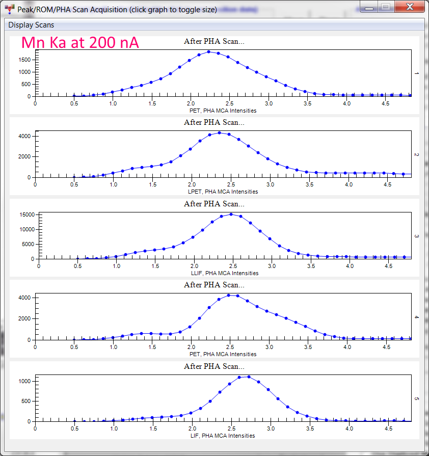
The LPET count rates were over 240K cps at 200 nA. Surprisingly good I think for an instrument with 3 usec dead times!  I'll try and remember to do a wavescan at 200 nA next time I'm in the lab, but again, the accuracy of the k-ratio data tells me that we are able to perform quantitative analysis at count rates never before attainable. 

If the counter is nearing paralysis, then, obviously, the Ti Ka count rate on Ti metal will produce this effect at lower current than TiO2.  This would be manifested as increasing positive deviation from rough linearity at high current on the plot of k-ratio versus current.  If I put a ruler up to your plot, then I can in fact see the apparent k-ratio deviating in this manner (but I need a ruler to see it).

When dealing with these high count rates, it really is necessary to specify whether the stated count rate is corrected or not (like the 506 kcps on Ti metal at 180 nA); this is one advantage of plotting against specified measured or corrected count rate rather than current.  On my channel 2/PETL, I see no obvious evidence for paralysis at 200 nA when measuring Ti Ka on high-purity TiO2 (with measured count rate between 250 and 300 kcps).  When I do a peak search at 400 nA to simulate the count rate on Ti metal, I get a peak with a distinctly flat top, indicating onset of paralysis.

Considering the above, it appears likely that your k-ratios collected above 140 nA are in fact affected by abnormal counter behavior, and so my first impression of the uncorrected ratios was wrong.  (But who could blame me considering that your plot contains no explicit information on measured count rate?)  What bothers me about your k-ratio versus current plots, though, is the fact that I can see patterns in the corrected values.  For instance, why do the corrected ratios for Anette’s channels 2 and 3 decrease in similar fashion when progressing from about 40 to 100 nA?  Why does a maximum appear to occur at 40 nA for the corrected channel 5 ratios?

I think that you need to investigate your model further to see if it is producing unphysical behavior.  I’ve already pointed out a potential problem on my N12/N32 versus N12 plot for Ti (shown again below).  It is absolutely physically impossible for N12/N32 to fall below the ratio determined in my linear fit, as this fit gives the extrapolation to zero count rate (noting that I collected abundant data in the linear region).  You or somebody else absolutely needs to test the higher order models in the same fashion.  Forming a ratio of Ti Ka and Ti Kb (with Kb measured on a spectrometer that produces relatively low count rate) is especially useful because the Kb count rate can be corrected reasonably with the linear model.  If you want to stick with k-ratios, then use a secondary standard that doesn’t contain much of the element under consideration (like Fe in bornite, Cu5FeS4, while using Fe metal as the primary standard).  On my plot of the uncorrected or linearly corrected data, note that no obvious deviation from linearity occurs below 85 kcps.

Well I'm glad you now see it.  And thank-you for taking the time to debate this with me. I have to say, all of this argument has actually helped me to appreciate exactly how good this new method and expression are.

The small deviations you point out are interesting and perhaps will provide additional insight into the inner workings of our instruments, but it should be noted that they are in the sub 1% level and significantly smaller than the k-ratio variations from one spectrometer to another.  The fact that we can attain 1% k-ratio accuracy up to 500K cps is, to me at least and Anette as well, the take home message in my book.

Here's an idea: I can't send you Anette's data until I ask her, but perhaps your best bet for understanding this constant k-ratio method and the new dead time expression is to perform a constant k-ratio run yourself. 

You already own Probe for EPMA, so why don't you just fire it up, go to the Help menu and update it to the latest version so you have the new dead time expression.  Then using Ti metal and TiO2, or any two materials with a large difference in count rates, try it out on your PET and LIF crystals.  Do you have any large area crystals? That is where these effects will be most pronounced. The procedure has been fully documented and is attached below.

Remember, Probe for EPMA has the traditional (single term) expression, the Willis (two term) expression, and the new six term expression, all available with a click of the mouse.  They are each simply more precise formulations of the probability calculation of randomly overlapping time intervals.


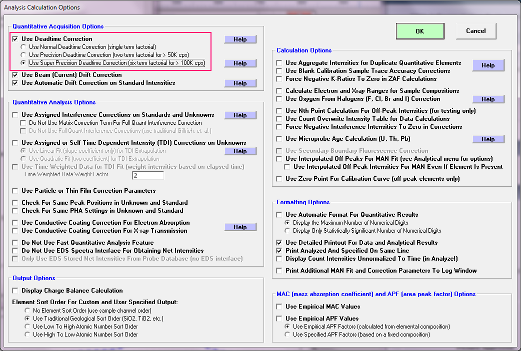
And by unchecking the Use Dead Time Correction checkbox you can even turn off the dead time correction completely!

With the latest version of Probe for EPMA, it just takes a few minutes to set up a completely automated overnight run using the multiple sample setups feature with different beam currents.  See the attached PDF document for complete details.

Edit by John: updated pdf attachment
« Last Edit: September 09, 2022, 08:22:17 AM by Probeman »
The only stupid question is the one not asked!