Generalized dead times

[sem-geologist]

And we come again at problem of PHA distribution shift... As Far as I could find out it is caused at least by two processes, where mild shift can be mitigated up to raw 100kcps (until other process kicks-in and overwhelms it with a real SHIFT of everything). Actually that correctable (mild) process is not shift at all - it is fortunately only downsizing of the pulse!

I had already posted those before but no one commented it... so look:

The description under the picture: Auto PHA sets low gain, and high bias (supposing that gas amplification produce less noise than semiconductor amplification (Please, have a bit more faith in modern electric engineering)). That at higher count rate causes slower charging step transition (longer delta t between cascades) at charge sensitive preamplifier's feedback capacitor (working closer to fully charged state) and signal further is translated by CR differentiator (OPAMP-based, called as Shapping Amplifier) to appear as lower amplitude pulse, than it would be seen at lower count rates.

So my mitigation for PHA downsizing problem is to lower the bias (and increase gain a lot, look - it is near Max (12-bits = 4096)  and then going up to 100kcps (raw counts) I don't need to touch any gain:


Now I am wondering how far such strategy could work for JEOL...

[Probeman]

And we come again at problem of PHA distribution shift... As Far as I could find out it is caused at least by two processes, where mild shift can be mitigated up to raw 100kcps (until other process kicks-in and overwhelms it with a real SHIFT of everything). Actually that correctable (mild) process is not shift at all - it is fortunately only downsizing of the pulse!

I see two effects in your plots above when going from low to high count rates, and also in my own data as shown here:

https://probesoftware.com/smf/index.php?topic=1466.msg11271#msg11271

First the downward shift in the PHA peak position at higher count rates and second the broadening of the right side of the peak also at higher count rates. Any idea why we start seeing that "shelf" on the right side at higher count rates?

Note also that I was able to keep both the bias and gain the same on my data from 10 to 200 nA, which for Mn Ka on Spc 2, LPET at 200 nA on Mn metal is 260 kcps!  For the purposes of calibrating the dead times I think we should try to keep both the bias voltage and the gain constant if possible (control our dependent variables!).

So why do you "mitigate" pulse height depression by decreasing the bias and increasing the gain (a lot)? What is your thinking on this? Why not simply keep the bias at a normal value and just increase the gain until the PHA peak is around 3 volts or so at a low count rate?  Then when the count rate is increased up to 260 kcps or more, the peak is still well above the baseline.  At least on Cameca instruments! 

Yes, the JEOL instrument may be unable to keep the bias voltage constant (over a large range of count rates) due to their very coarse gain settings, but why change the bias voltage at all on the Cameca?

I am not using auto PHA, because I want to adjust things manually. May we see your PHA scans at count rates greater than 100 kcps?

Now I am wondering how far such strategy could work for JEOL...

Good question.  To add some data to our speculations, here are some PHA scans from Anette's most recent run. First here is a normal TAP spectrometer at 10 nA:



and now at 120 nA:



Not very pretty I know, but if JEOL's integral mode works as expected(?) we are hopefully not losing any counts on the high side. By the way, the above PHA scan was on Si metal and extrapolating from 10 nA should have a predicted count rate of around 334 kcps at 120 nA. 

Now let's look at the TAPL crystal (hold on to your seats!), first at 10 nA:



and now at 120 nA:



Pretty ugly but at least the PHA peak is above the baseline!  By the way, again extrapolating from 10 nA, the predicted count rate for this TAPL crystal at 120 nA is 894 kcps!!!!

[sem-geologist]

I see two effects in your plots above when going from low to high count rates, and also in my own data as shown here:

https://probesoftware.com/smf/index.php?topic=1466.msg11271#msg11271

First the downward shift in the PHA peak position at higher count rates and second the broadening of the right side of the peak also at higher count rates. Any idea why we start seeing that "shelf" on the right side at higher count rates?

shift, broadening and "shelf" are due to same process - pulse pileup, I already discussed that it in other posts. So sorry from repeating myself. "Shelf" represents the double piled up peaks (thus double energy). The Broadening is by imperfect positive and negative+positive pileups dominating the part of pileuped pulses, in my case also Ar esc pulses pileup with every other pulse combinations (as it is Ti Ka). shift is due to pulses being bi-polar (bipolar pulse: voltage raises to positive voltage, then it goes down and overshots the 0V going into wide negative voltage forming the negative tail slowly getting back to 0V) and its negative tail being much longer than positive pulse - with increased pileup many pulses starts at such negative tail, or double-deep negative tail or even more - thus PHA sees a shift as a function of increased pulse density (as PHA measures difference of voltages between top of pulses and 0V).

So why do you "mitigate" pulse height depression by decreasing the bias and increasing the gain (a lot)? What is your thinking on this? Why not simply keep the bias at a normal value and just increase the gain until the PHA peak is around 3 volts or so at a low count rate?  Then when the count rate is increased up to 260 kcps or more, the peak is still well above the baseline.  At least on Cameca instruments! 

1) This mitigation is very beneficial for differential PHA mode for higher order line minimization (elimination is impossible up to 4th order, with current hardware - thus only minimization)! 2) Lower bias will age the counter slower! 3) there is actually no normal values - You get exactly the same amount of counts with lower bias and high gain compared with lower gain higher bias using integral mode - thus there is no normal values - they are canonical - they are settled so by tradition of fear - fear of analog electronics noise. Well there is actually the lower threshold how much bias can be dropped, where below that value it will start to decrease the count rate. For high pressure spectrometers that should not be below 1600-1650 V (for Cameca spectrometers), the threshold can be experimentally found by setting max gain, and changing bias until the raw count rate starts to drop. The shared PHA demonstration was pushed to extreme (very near the threshold) to showcase the mitigation of the "Pulse amplitude downsizing by increased average load in feedback capacitor of Charge Sensitive Preamplifier".

[Probeman]

I see two effects in your plots above when going from low to high count rates, and also in my own data as shown here:

https://probesoftware.com/smf/index.php?topic=1466.msg11271#msg11271

First the downward shift in the PHA peak position at higher count rates and second the broadening of the right side of the peak also at higher count rates. Any idea why we start seeing that "shelf" on the right side at higher count rates?

shift, broadening and "shelf" are due to same process - pulse pileup, I already discussed that it in other posts. So sorry from repeating myself. "Shelf" represents the double piled up peaks (thus double energy). The Broadening is by imperfect positive and negative+positive pileups dominating the part of pileuped pulses, in my case also Ar esc pulses pileup with every other pulse combinations (as it is Ti Ka). shift is due to pulses being bi-polar (bipolar pulse: voltage raises to positive voltage, then it goes down and overshots the 0V going into wide negative voltage forming the negative tail slowly getting back to 0V) and its negative tail being much longer than positive pulse - with increased pileup many pulses starts at such negative tail, or double-deep negative tail or even more - thus PHA sees a shift as a function of increased pulse density (as PHA measures difference of voltages between top of pulses and 0V).

OK, thanks. That sounds quite reasonable. And I note that we see the same sort of "shelving" in the JEOL PHA scans at higher count rates, even though the peaks are much broader for some reason:

https://probesoftware.com/smf/index.php?topic=1489.msg11281#msg11281

Any idea why the JEOL PHA peaks are so broad?

So why do you "mitigate" pulse height depression by decreasing the bias and increasing the gain (a lot)? What is your thinking on this? Why not simply keep the bias at a normal value and just increase the gain until the PHA peak is around 3 volts or so at a low count rate?  Then when the count rate is increased up to 260 kcps or more, the peak is still well above the baseline.  At least on Cameca instruments! 

1) This mitigation is very beneficial for differential PHA mode for higher order line minimization (elimination is impossible up to 4th order, with current hardware - thus only minimization)! 2) Lower bias will age the counter slower! 3) there is actually no normal values - You get exactly the same amount of counts with lower bias and high gain compared with lower gain higher bias using integral mode - thus there is no normal values - they are canonical - they are settled so by tradition of fear - fear of analog electronics noise. Well there is actually the lower threshold how much bias can be dropped, where below that value it will start to decrease the count rate. For high pressure spectrometers that should not be below 1600-1650 V (for Cameca spectrometers), the threshold can be experimentally found by setting max gain, and changing bias until the raw count rate starts to drop. The shared PHA demonstration was pushed to extreme (very near the threshold) to showcase the mitigation of the "Pulse amplitude downsizing by increased average load in feedback capacitor of Charge Sensitive Preamplifier".

I get that this would reduce spectral interferences from high order reflections, but why not just use the spectral interference correction in PeakSight?

I know the interference correction in PeakSight a bit of a pain to use compared to quantitative interference correction in Probe for EPMA, but at least it provides a full correction for all interferences including first order interferences.

https://probesoftware.com/smf/index.php?topic=69.0

My advice to all my users and students is: adjust your PHA gain so the peak is well centered (maybe slightly to the left of center on a high concentration standard, so the there's room for it to shift to the right at lower count rates), and use integral mode and keep the baseline under 0.5 volts.  This way the spectrometer response will be quite linear no matter what the count rate is.

In other words, let all the x-rays in, and correct for spectral interferences as God intended      using a quantitative interference correction:

https://probesoftware.com/smf/index.php?topic=69.msg1189#msg1189

Having a linear spectrometer response is of course essential for the constant k-ratio calibration for dead time:

https://probesoftware.com/smf/index.php?topic=1466.msg11102#msg11102

Have you had a chance to acquire some constant k-ratios on your instruments?

[sem-geologist]

Any idea why the JEOL PHA peaks are so broad?

Because by increasing bias for keeping the main PHA peak at the same position it actually makes "zooming-in" like procedure (increasing Gain actually would do the same zooming magic). Increasing bias increases amplification and increases the real amplitude of Pulses. The thing which hides this is that both Cameca And Jeol PHA measures not real amplitude of pulse, but voltage from top of peak in reference to 0V (where pulse often at high count rate can start at negative voltage). So lets say Pulse is 5V height +/- 0.5V (at small count rate, the chosen values are for demonstration, not at exact proportions seen on instruments). At very high rate such most common pulse starts at ~ -2.5V and PHA measuring its top sees (and plots) only 2.5V plus the spread is still similar +/- 0.5V. Now Jeol User will increase bias to move that 2.5V PHA peak to be "back" on 5V. What happens behind the Users observable PHA graphs and slips unnoticed behind his back is that amplitude of pulse just was increased twice around the 0V to both sides (+V and -V) symmetrically (increasing those negative after-pulse tails (and thus whole part of signal at negative to 0V). So then at such high count rate pulses start no more at average of -2.5V but at average at -5V. So real amplitude was increased twice (from 5V to 10V), and so the distribution looks like broadening as that is zooming in and that initial uncertainty of +/- 0.5V got enlarged twice as well into +/- 1V. So as the end result The user having no idea that base line of pulses are far away in negative voltage sees the same centered pulse but much broader 5V +/-1V. And of course pile ups adds some more broadening on that.

I get that this would reduce spectral interferences from high order reflections, but why not just use the spectral interference correction in PeakSight?

I know the interference correction in PeakSight a bit of a pain to use compared to quantitative interference correction in Probe for EPMA, but at least it provides a full correction for all interferences including first order interferences.

https://probesoftware.com/smf/index.php?topic=69.0

The pain? I would argue that it is not so much (especially that I have some (own written) software to manage interference corrections, and can construct the set of corrections for new setup or evaluate validity for modified... my interference corrections often gets like ~50-100 corrections and above that (max has 150 for 43 elements)). Yes Peaksigh has some pain with circular correction... which can be worked around very easily. But my most liked feature which is in Peaksight 6.5 is its ability to handle negative interference (interference with background measurements) - which works remarkably. And so I was on the same boat: "Don't use narrow window diff, use interference corrections on all orders... for correction".  However I came across some experience which changed my mind. This year I adapted measuring the Si, Mg, and Al on second order lines (which worked remarkably at the beginning) but after getting back to work after vacation I had found out that after changing of season the intensities had dropped tens of percent (!), while intensities of first order stayed comparably same. I then started searching for answer if higher diffraction order intensities depends from some physical factors. I even asked this question on Research Gate:
https://www.researchgate.net/post/Can_proportion_of_intensities_of_different_orders_from_diffracted_X-rays_depend_on_temperature

There answer is IT DOES! And that would then require to do often calibration of such interference corrections (for higher order lines) that brings an additional hassle, but that would be not practical as it can change during the day when high precision trace element compositions are measured. I was wondering why my Monazite Dating floats at summer from older at evening to younger toward next morning - I was doing interference correction of 2nd and 3rd order lines of REE for U,Th,Pb. After I ditched that, and moved to diff mode for these elements - analyses started to be stable and no more produce any clear daily biases.

[Probeman]

Any idea why the JEOL PHA peaks are so broad?

Because by increasing bias for keeping the main PHA peak at the same position it actually makes "zooming-in" like procedure (increasing Gain actually would do the same zooming magic). Increasing bias increases amplification and increases the real amplitude of Pulses. The thing which hides this is that both Cameca And Jeol PHA measures not real amplitude of pulse, but voltage from top of peak in reference to 0V (where pulse often at high count rate can start at negative voltage). So lets say Pulse is 5V height +/- 0.5V (at small count rate, the chosen values are for demonstration, not at exact proportions seen on instruments). At very high rate such most common pulse starts at ~ -2.5V and PHA measuring its top sees (and plots) only 2.5V plus the spread is still similar +/- 0.5V. Now Jeol User will increase bias to move that 2.5V PHA peak to be "back" on 5V. What happens behind the Users observable PHA graphs and slips unnoticed behind his back is that amplitude of pulse just was increased twice around the 0V to both sides (+V and -V) symmetrically (increasing those negative after-pulse tails (and thus whole part of signal at negative to 0V). So then at such high count rate pulses start no more at average of -2.5V but at average at -5V. So real amplitude was increased twice (from 5V to 10V), and so the distribution looks like broadening as that is zooming in and that initial uncertainty of +/- 0.5V got enlarged twice as well into +/- 1V. So as the end result The user having no idea that base line of pulses are far away in negative voltage sees the same centered pulse but much broader 5V +/-1V. And of course pile ups adds some more broadening on that.

So you are saying that the reason for the apparent broader PHA peaks on JEOL instruments is due to the fact that the JEOL electronics amplifies the pulse distribution to 0 to 10v, while Cameca only amplifies to 0 to 5v?

And are you also saying there is more pulse pileup on JEOL instruments (and therefore more peak broadening)? Could some of that be due to the JEOL spectrometer's larger geometric efficiency from having the smaller focal circle? Or is it mostly that the JEOL electronics is faster and therefore it sees more raw counts?

I posted this comparison between JEOL and Cameca instruments here looking at the raw observed count rates as a function of beam current:

https://probesoftware.com/smf/index.php?topic=1489.msg11277#msg11277

In your response to that post you mentioned setting the hardware (integer) dead times to 1 usec on your Cameca instrument, and seeing many more counts at high beam currents.  But in the past when I've set my hardware (integer) dead times to 1 usec, I still measured dead times around 2 usec or so, which is why I think the Cameca is intrinsically a higher dead time system than the JEOL.

Attached are spreadsheets I did many years ago testing the dead times when the hardware was set to 1 usec for Si ka and Ti ka on Si metal and Ti metal.  The measured dead times were around 2 for both x-rays.

But maybe this is all moot, as we wouldn't want to run without imposed (hardware) dead times of 3 usec, correct?  I believe you also run using a hardware integer dead time of 3 usec? 

That said, I am trying to remember when we upgraded our WDS board, as these tests were performed in 2010!  I think we upgraded our stage and WDS boards when we got v. 4.2 of PeakSight, so when was that released?  Maybe I should re-run some dead time calibrations with the new WDS board using new constant k-ratio method with the hardware dead times set to 1 usec just to see if I get similar numbers as before?   

I'll try sneaking into the lab this weekend if the instrument isn't busy!   

[sem-geologist]

So you are saying that the reason for the apparent broader PHA peaks on JEOL instruments is due to the fact that the JEOL electronics amplifies the pulse distribution to 0 to 10v, while Cameca only amplifies to 0 to 5v?

No I am not saying that. Where had you got this from? I am saying the broadening is because of "zooming" effect.

I think You fail to grasp what is bipolar-pulse and its importance for observed artifacts with increasing density of pulses (increasing count rates). I already uploaded in few places oscilloscope screenshot, but maybe it is overwhelming.  So I am stopping here and can go further with explanation only If I am sure You understand the bipolar pulse. I am extremely bad on sketching, please find below the part of simplified sketch showing how bipolar pulse is born (in WDS G(F)PC pulse forming).

So look to this (I am also attaching it as vector version in attachments); (PS.: only bipolar pulse presented below has a very precise shape as that is pulse being measured with oscilloscope, other earlier forms of pulse in pipeline are reconstructed from it):

[Probeman]

So you are saying that the reason for the apparent broader PHA peaks on JEOL instruments is due to the fact that the JEOL electronics amplifies the pulse distribution to 0 to 10v, while Cameca only amplifies to 0 to 5v?

No I am not saying that. Where had you got this from? I am saying the broadening is because of "zooming" effect.

I think You fail to grasp what is bipolar-pulse and its importance for observed artifacts with increasing density of pulses (increasing count rates). I already uploaded in few places oscilloscope screenshot, but maybe it is overwhelming.  So I am stopping here and can go further with explanation only If I am sure You understand the bipolar pulse. I am extremely bad on sketching, please find below the part of simplified sketch showing how bipolar pulse is born (in WDS G(F)PC pulse forming).

So look to this (I am also attaching it as vector version in attachments); (PS.: only bipolar pulse presented below has a very precise shape as that is pulse being measured with oscilloscope, other earlier forms of pulse in pipeline are reconstructed from it):

OK, then are you saying that the Cameca instrument performs an extra step of converting from mono-polar to bipolar pulses, that the JEOL electronics does not?  And that is the reason for the thinner PHA peaks on the Cameca pulse processing electronics?

Sorry if I ask dumb questions, I am not familiar at all with these electronic details.

[sem-geologist]

OK, then are you saying that the Cameca instrument performs an extra step of converting from mono-polar to bipolar pulses, that the JEOL electronics does not?  And that is the reason for the thinner PHA peaks on the Cameca pulse processing electronics?

Sorry if I ask dumb questions, I am not familiar at all with these electronic details.

Those are not dumb questions, those are actually very valid questions, just  a bit in this context inpatient like "a-cart-attached-before-the-horse". The answer is, unless someone would invite me to peek into Jeol Probe electronics (at least to detector electronics), it is hard to tell.

So if we open the case where the Shapping of pulse takes place we see this (My kind reminder: DEADLY high voltage is present on part of such board):

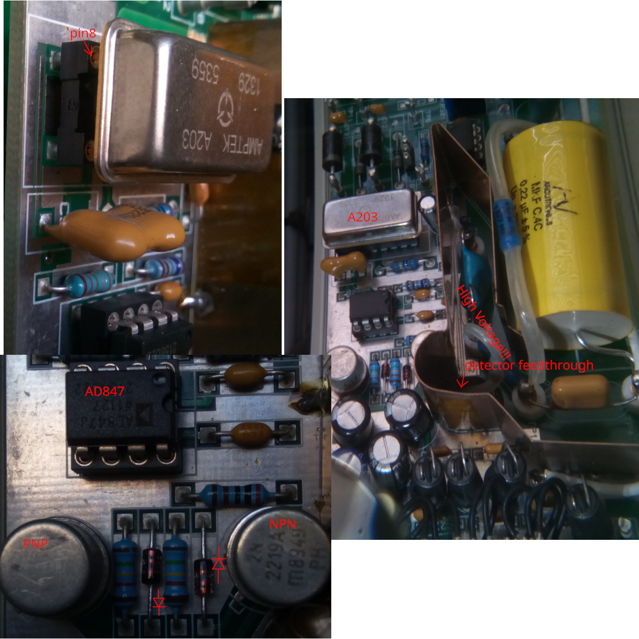
The Charge-Sensitive Preamplifier (CSP) and the Shapping Amplifier (SA) are packed inside single a single chip produced by Amptek - A203. The SA on that chip offers both: bipolar (pin9) and unipolar (pin8) outputs, however from visual inspection it is clear that Cameca uses unipolar (pin8, a clear trace from it, then around A203 to the capacitor for decoupling, which is required by documentation of A203) output from that chip and by components placed on the shielded ground plane (which points to very careful design for sensitive signal handling) it is clear that it does the 2nd differentiation on its own implementation (with OPAMP AD847). But why? I believe it is as A203 is not able to drive terminated (75ohm) coaxial cable on its own as A203 bipolar output is rated for 2kohm impedance - connecting such signal directly to terminated coaxial (75ohm) would lower down the amplitude a lot (x30 times), thus I think Cameca uses its own implementation with 2nd differentiation of monopolar pulses and (what I suspect from clearly visible two diodes and connection with NPN and PNP transistor pair) signal after that differentiation goes through class AB power amplifier (the short explanation what it is: https://www.elprocus.com/class-ab-amplifier/) as signal needs to be driven through few meter terminated coaxial cable to the gain and counting electronics. Just a side note: there are hardly any high speed OPAMPS which could directly drive such loads at these voltages (+/-15V), and thus the engineering of Cameca in this regard is a top notch.

So to answer the question if Jeol "shortcuts" on signal handling and thus PHA distribution suffers because of that - that would need similar inspection on Jeol hardware side: We need to know, what CPS and SA it uses (i.e. A203 is unique in its integration of both CSP and SA into single package - but it is possible to use separate CSP and SA chips (i.e. produced by Cremat inc.) to get the similar functionality), what kind of coaxial cable is used to send the signal from detector to counting board. Design for a few hundred of thousands of pulses a second is not complicated. However with Million pulses in second a single weak point in design can cause the amplitude drop.

This 75 ohm terminated coaxial cable is making me a headache for my planned experiment with external pulse generator. This means I will need to implement some fast class AB power amplifier if I want to simulate the pulses from the above presented circuit.

I however am skeptical if above described part of pipeline would produce observed differences in severity of PHA shift and broadness on Jeol probes. I introduced the description of bipolar pulse as a starting point to go further with explanation what happens next - when density of such pulses increase (count rate increase). We also can see the PHA shift on Cameca instruments and PHA distribution goes straight to hell when going to very high input count rates (like >1Mcps). And PHA shifting if using normal bias values is visible already from 20kcps and up.

So at first I want to present how I know the PHA shifts are produced on Cameca WDS hardware and in particular - how the bipolarity of pulses is causing that. Also my presented mitigation for "downsizing" (not to mistake with PHA shift) has a part in this story, and knowing if early shift can be mitigated by lowering the bias and increasing the gain can shed some light why Jeol PHA has more severe shifts (and broadening). I guess that there is not much difference of how Cameca converts unipolar to bipolar (doing math differentiation with OPAM), but how unipolar pulses looks like and differs by different handling of SA and CSP used by these two vendors. Unfortunately everything in pipeline before the bipolar pulse is more theoretical, as only bipolar output can be captured with oscilloscope. Nevertheless, knowing the process it is possible to reconstruct earlier shapes in the pipeline and find the possible reason even without opening the case and looking to the physical components of electronics.

[Probeman]

OK, then are you saying that the Cameca instrument performs an extra step of converting from mono-polar to bipolar pulses, that the JEOL electronics does not?  And that is the reason for the thinner PHA peaks on the Cameca pulse processing electronics?

Sorry if I ask dumb questions, I am not familiar at all with these electronic details.

Those are not dumb questions, those are actually very valid questions, just  a bit in this context inpatient like "a-cart-attached-before-the-horse". The answer is, unless someone would invite me to peek into Jeol Probe electronics (at least to detector electronics), it is hard to tell.
...
So to answer the question if Jeol "shortcuts" on signal handling and thus PHA distribution suffers because of that - that would need similar inspection on Jeol hardware side...

OK, so I assume your answer is: we do not know yet...

We would still love to see some constant k-ratio data from your instruments. You saw the data from Jlmaner87's tactis instrument here?

https://probesoftware.com/smf/index.php?topic=1466.msg11238#msg11238

Login to see attachments...

[sem-geologist]

OK, so I assume your answer is: we do not know yet...

We would still love to see some constant k-ratio data from your instruments. You saw the data from Jlmaner87's tactis instrument here?

https://probesoftware.com/smf/index.php?topic=1466.msg11238#msg11238

Login to see attachments...

Yes we don't know yet, however understanding what causes PHA shifts on Cameca instruments can point where to look exactly on Jeol probes.

Also Yes I saw these k-ratio data. Unfortunately our SXFive is heavily booked, hopefully soon there will be some time window for such measurements.

[Probeman]

Now I need to change my dream instrument somewhat from:

https://probesoftware.com/smf/index.php?topic=1410.msg10366#msg10366

to:

1. JEOL FEG electron column

2. Cameca WDS spectrometers with linear optical encoding

3. Bruker or Thermo SDD EDS

4. Cameca stage with linear optical encoding

5. Cameca light optics

6. Cameca pulse processing electronics with JEOL dead times

7. Polycold cryo-pumped vacuum baffle (100 Kelvin) with turbo pump

 

[sem-geologist]

Now I need to change my dream instrument somewhat from:

https://probesoftware.com/smf/index.php?topic=1410.msg10366#msg10366

to:

1. JEOL FEG electron column

2. Cameca WDS spectrometers with linear optical encoding

3. Bruker or Thermo SDD EDS

4. Cameca stage with linear optical encoding

5. Cameca light optics

6. Cameca pulse processing electronics with JEOL dead times

7. Polycold cryo-pumped vacuum baffle (100 Kelvin) with turbo pump

 

1. What so good with Jeol FEG and what so bad with Cameca FEG? Cameca FEG if run correctly can be stable as it can get (<0.5% 24h). I had hear lots of not so good rumors about Jeol column stability. If I would need to consider dream instrument for this point my choise of FEG would be Shimadzu one, as looks they are the first to understand the real advantage of FEG for EPMA (stability and very high current, or at least addresses correctly those advantages in the marketing, and states that they use a bit bigger FEG than SEM which mean easier attainable ultimate Stability).

6. Also why do You think You need Jeol dead times? If there is not enough counts, and You want to see also much bigger PHA position swing, then set Hardware dead time to 1µs (I suppose You had not redone the test and are using default 3µs) and enjoy.

[Probeman]

1. What so good with Jeol FEG and what so bad with Cameca FEG? Cameca FEG if run correctly can be stable as it can get (<0.5% 24h). I had hear lots of not so good rumors about Jeol column stability. If I would need to consider dream instrument for this point my choise of FEG would be Shimadzu one, as looks they are the first to understand the real advantage of FEG for EPMA (stability and very high current, or at least addresses correctly those advantages in the marketing, and states that they use a bit bigger FEG than SEM which mean easier attainable ultimate Stability).

That is not what I hear from Cameca FEG owners. I hear that if they try and change the beam current they have to wait a long time for stability to return.  I also hear that the electrostatic beam blanker introduces additional instability.  Anyway, it's all moot now since Cameca is going to stop producing EPMA instruments. At least any instruments that most of us can afford!

6. Also why do You think You need Jeol dead times? If there is not enough counts, and You want to see also much bigger PHA position swing, then set Hardware dead time to 1µs (I suppose You had not redone the test and are using default 3µs) and enjoy.

Aren't you using an enforced dead time of 3 usec on your instrument? My view is that the less dead time the better, especially for high speed quantitative mapping using high beam currents.  The smaller the dead time correction, the better is my thinking.  I hope we all agree that SDD detectors/electronics with 1/10th dead times are better than Si(Li)? 

I will try and run a 1 usec enforced test again this weekend using the constant k-ratio method:

https://probesoftware.com/smf/index.php?topic=1466.msg11102#msg11102

[sem-geologist]

Aren't you using an enforced dead time of 3 usec on your instrument? My view is that the less dead time the better, especially for high speed quantitative mapping using high beam currents.  The smaller the dead time correction, the better is my thinking.  I hope we all agree that SDD detectors/electronics with 1/10th dead times are better than Si(Li)? 

No, I am moving away from 3µs: and moving any new calibrations for new analysis to 1µs if using PHA integral mode, and also enlarging the dead time to 5µs if going for narrow window PHA diff mode (also reducing bias, not so extreme as in my example above, (i.e. just down to 1700 V from 1850, and increasing gain accordingly), as 3µs is not enough to get back from pulse depression to 0V of those bipolar pulses. 3µs is safe value (and I am still not going below on our SX100 with old WDS board), but not optimal for different purposes especially on new machines - and the ability left to user to set it to this or that value gives flexibility. The Peaksight has only a single dead time correction model (nothing so fancy as PfS) and thus moving to 1µs makes even not perfect dead time correction messing up things less.

Well, Cameca FEG... to be honest I was mad about it too in the beginning as we had different expectations. For sure stability-wise it is less flexible than Tungsten based SX. You can't just jump up and down with HV and current, and that can be worked around with better planning with analytical strategy (i.e. doing 10nA, then 20nA, then 200nA) and merge these after acquisition.

However, the most wickedest thing I find with that column is the splash aperture mounted in a way that replacement needs basically dismantling upper part of the column - that is my most hated thing with that design and that IMHO is the main source of instabilities observed later even if FEG is well maintained (like after one year of using, which after 2 years of using it basically blocks using the HV <12kV, as contamination on that aperture is able to deflect the beam).

The normal apertures fortunately can be easily changed as in SX100. I also found out that with FEG it is much better to let go the beam regulator (I am not using that at all) as not regulated beam is much more stable (I saw also Theo not long ago asked how to use PfS with 200µm not regulated aperture, probably found out the gotcha too). I can not comment on stability of electrostatic lens - actually I have no complaint about that and can't get how any proof that it cause any instability can be gathered. Contrary, I think the problem with instabilities lies with instability caused by too heavy reliance on single condenser lens, which alone needs to to handle such different power loads compared to the set of two lenses on W/LaB6 column. In example its power (C2) needs to be decreased in about ~70% of full range to go from 1pA to 800nA (on single aperture),  where two-lens system changes power only 15-20% for that. And thus it is rather thermal re-equilibration of lenses (and its power supply circuit) which cause instabilities then changing the beam current, but that can be mitigated easily by using more different apertures, allowing to stay within similar range of C2 power (using 70µm aperture for low beam currents and 200µm aperture for high currents). Our current FEG tip is running already 3.5 years and still kicking (still able to provide maximum 1000nA with 0.5% stability, i.e. Zr in Rutile enjoys these tickling currents, unless it is grains in epoxy - epoxy expands terribly and 1) cracks  and 2) surface goes out of focus)!