Unfortunately I had no time to do that k-ratio test (it is time consuming) and our machine is kept occupied even at weekends (which makes me very happy). Hopefully, there will be a short window in the schedule next week.
However, I was not idle, and done some more interesting prep and modeling work for future experimentation, and came up with some more (important for dead time) ideas to check in the future. If you remember I had mentioned some artificial signal generator. I already got raspberry pi nano (what an incredible capable small board for a few bucks), played around with R2R (resistor ladder) 8 bit DIY DAC firstly on breadboard (which I found is junk), and after moved to soldered assembly. 8-bit DAC works nicely, but before I can connect that to coaxial cable (with 75ohm termination) of WDS signal, I need to amplify and shift the Voltage level (This Rpi nano and DAC is outputing signals 0V/+3.29V, and I need to scale that to -15V/+15V, or at least -12V/+12V) and amplify the power. I somehow initially bought pretty cheap OPAMP which is capable only up to 3Mhz. Ideally I should buy the same AD847 (type used in original signal processing), but there is issues with supply chain, and it is quite expensive. But I start to doubt if that would not be an overkill...
Anyway, I also was working on the way to demonstrate as much as clear why bipolar pulses and its bipolarity maters (how it is behind the shifting and broadening of the PHA distribution). So I took this picture which I already showed previously as a starting point:
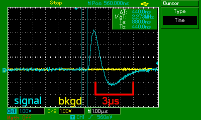
and prepared it for capturing the waveform (the time section of 12µs has 300pixels, thus one pixel = 40ns). I refined the captured shape (the orange curve) until integration of the bipolar-pulse (the previous -unipolar- form (blue curve)) would begin at 0=0 and end at y=0:

As we can see from that picture the properties of asymmetry (around y=0) of bipolar pulse is inherited from asymmetry (around x) at max position of uni-polar pulse - its left side is shorter than right side. Unipolar pulse gets its asymmetry from "cascade" pulses and the background of Charge sensitive preamplifier. Thus important questions are:
Would Unipolar pulse look the same at very high count rates, and low count rates? Would not slope of background should be different - and thus tail - and so the shape of bipolar pulse? The longer is the tail, the longer is the negative part of bipolar pulse, and the shallower.
...so, should unipolar end at y=0 at all count rates or rather not at all???
edit: answer after comparing pulses from measurements on low count rate and high count rate is - it does not change the shape.I am attaching the digitized form of pulse below as txt.
I found out that it is very easy to model pulse coincidences using simple numpy library of python, using ".convolve" method.
I am not adding any units (neither y, neither x is so important, the important is only pulse proportions), as if I would introduce U [V] and t[µs] and then probeman would freak out that this has something to do with electronics

, so I leave these unit-less. Also my in-construction pulse generator will be using 8-bit values - thus I will confuse less myself keeping this like that.
So first to import the pulse shape we do:
import numpy as np
import matplotlib.pyplot as plt

bi_pulse_model = np.loadtxt("SX_pulse_model_40ns.txt")
plt.plot(bi_pulse_model)
plt.show()
to get the previous unipolar form we need to do integration of signal:
uni_pulse_model = np.cumsum(bi_pulse_model)
plt.plot(bi_pulse_model * 10, label="bipolar")  # lets scale for comparison with unipolar pulse
plt.plot(uni_pulse_model, label="unipolar")
plt.legend()
plt.show()
But that alone, while is interesting, is not so useful.
The real interesting part starts when we define some longer time space in example 1000 units (the pulse model between points is 40 ns; such 1000 units would represent 40µs)
pulse_space = np.zeros(1000)
in example if we want pulses every 4µs:
pulse_space[0::100] = 1
Then we can convolute pulses on this like that simple:
model = np.convolve(pulse_space, bi_pulse_model)
plt.plot(model)
plt.show()
which would produce this (for 250kcps):

And so if we start to decrease this gap between pulses we start to see amplitude (Relative to y=0) shift downward (except the very first pulse):
pulse_space[:] = 0 # reset everything to 0
pulse_space[0::75] = 1 # pulse every 3µs
model = np.convolve(pulse_space, bi_pulse_model)
plt.plot(model)
plt.show()
which would produce this for 3µs (for 333kcps):

then for 2µs after code modification (for 500kcps):

then for 1µs (for 1Mcps):

and finaly for 520ns (for 2Mcps):

Well, few things to remind - this is synthetic modeling with even time gaps between pulses imitating average time gap shortening with increased count rate. However pulses comes at random in real life. This simulation shows that with even spaced pulse trains PHA shift should start at 250kcps (input rate), however in real life we observe on Cameca it much earlier, because pulses randomly hit the spot close after other pulse. However this agrees quite well with breaking point of clear PHA shift increase crossing the 250kcps (input).
One more point is that those pulse trains are shifted with whole information of amplitude preserved. That gets clear with last negative big pulse when compared with y-shifted single pulse overlays. In example below, the previous (with gaps of 520ns) plot is zoomed at the end part of pulse train:

Stay tuned for the random pulse simulation.


 We depend on your feedback and ideas!