Author Topic: New method for calibration of dead times (and picoammeter)  (Read 23151 times)

Probeman

  • Emeritus
  • *****
  • Posts: 2831
  • Never sleeps...
    • John Donovan
Re: New method for calibration of dead times (and picoammeter)
« Reply #60 on: July 23, 2022, 09:26:05 AM »
Now that we have implemented Aurelien Moy's logarithmic expression let's see how it performs.

Here is a plot of observed vs. predicted count rates at 1.5 usec up to 300K observed count rates:


Wait a minute, where did the six term (red line) expression go?  Oh, that's right, it's underneath the log (cyan) expression. At under 300K cps observed count rates, these two expressions give almost identical results.  Meanwhile the traditional expression gives a predicted count rate that is about 30% to 40% too low!    :o

OK, let's take it up to 400K cps observed count rates:


Now we are just barely seeing a slight divergence between the two expressions which makes sense since the six term Maclaurin-like expression is only an approximation of the probabilities of multiple photon coincidences.

Note that at 1.5 usec dead times this 400K cps observed count rate corresponds to a predicted (true) count rate of over 4000K cps. Yes, you read that right, 4M cps. 

Of course our gas detectors will be paralyzed long before we get to such count rates.  From Anette's WDS data we think this is starting to occur at predicted (true) count rates of over 500K cps, which at 1.5 usec corresponds to an observed count rate of around 250K cps.

But even at these easily attainable count rates, the traditional expression is still off by around 25% relative.   It's all a question of photon coincidence.    :)
« Last Edit: July 23, 2022, 12:39:55 PM by Probeman »
The only stupid question is the one not asked!

Probeman

  • Emeritus
  • *****
  • Posts: 2831
  • Never sleeps...
    • John Donovan
Re: New method for calibration of dead times (and picoammeter)
« Reply #61 on: August 08, 2022, 10:22:07 AM »
Over the weekend I went over my MgO/Al2O3/MgAl2O4 consensus k-ratios from May, now that we finally figured out the issues with calibrating our WDS spectrometer dead times using the "constant k-ratios" procedure developed by John Donovan and John Fournelle and also attached to this post as a short pdf file:

https://probesoftware.com/smf/index.php?topic=1466.msg11008#msg11008

and now that we have an accurate expression for dead time correction (see Moy's logarithmic dead time correction expression in Probe for EPMA), we can re-open that old probe data file from May and re-calculate our k-ratios!

So, using the new logarithmic expression we obtain these k-ratios for MgAl2O4 from 5 nA to 120 nA:


Note that I blanked out the y-axis values so as not to influence anyone (these will be revealed later once Will Nachlas has a better response rate from the first FIGMAS round robin!) but the point here is to note how *constant* these consensus k-ratios are over a large range of beam currents.
 
What does this mean?  It means we can quantitatively analyze for major elements, minor elements, and trace elements at high beam currents at the same time!

This is particularly important for high sensitivity quantitative X-ray mapping...
« Last Edit: August 08, 2022, 10:47:47 AM by Probeman »
The only stupid question is the one not asked!

Probeman

  • Emeritus
  • *****
  • Posts: 2831
  • Never sleeps...
    • John Donovan
Re: New method for calibration of dead times (and picoammeter)
« Reply #62 on: August 08, 2022, 10:50:53 AM »
I almost forgot to post this.  Here's the analysis of the above MgAl2O4 using MgO and Al2O3 as primary standards, first at 30 nA:

St 3100 Set   3 MgAl2O4 FIGMAS
TakeOff = 40.0  KiloVolt = 15.0  Beam Current = 30.0  Beam Size =   10

St 3100 Set   3 MgAl2O4 FIGMAS, Results in Elemental Weight Percents
 
ELEM:       Mg      Al       O
TYPE:     ANAL    ANAL    SPEC
BGDS:      EXP     EXP
TIME:    60.00   60.00     ---
BEAM:    29.85   29.85     ---

ELEM:       Mg      Al       O   SUM 
    28  17.063  37.971  44.985 100.020
    29  17.162  38.227  44.985 100.374
    30  17.234  38.389  44.985 100.608

AVER:   17.153  38.196  44.985 100.334
SDEV:     .086    .210    .000    .296
SERR:     .050    .121    .000
%RSD:      .50     .55     .00

PUBL:   17.084  37.931  44.985 100.000
%VAR:      .41     .70     .00
DIFF:     .069    .265    .000
STDS:     3012    3013     ---

And here at 120 nA:

St 3100 Set   6 MgAl2O4 FIGMAS
TakeOff = 40.0  KiloVolt = 15.0  Beam Current = 120.  Beam Size =   10

St 3100 Set   6 MgAl2O4 FIGMAS, Results in Elemental Weight Percents
 
ELEM:       Mg      Al       O
TYPE:     ANAL    ANAL    SPEC
BGDS:      EXP     EXP
TIME:    60.00   60.00     ---
BEAM:   119.71  119.71     ---

ELEM:       Mg      Al       O   SUM 
    55  17.052  37.617  44.985  99.654
    56  17.064  37.554  44.985  99.603
    57  17.083  37.636  44.985  99.704

AVER:   17.066  37.602  44.985  99.654
SDEV:     .016    .043    .000    .051
SERR:     .009    .025    .000
%RSD:      .09     .11     .00

PUBL:   17.084  37.931  44.985 100.000
%VAR:     -.10    -.87     .00
DIFF:    -.018   -.329    .000
STDS:     3012    3013     ---

This is using the default Armstrong phi/rho-z matrix corrections, but all the matrix expressions give similar results as seen here for the 30 nA analysis:

Summary of All Calculated (averaged) Matrix Corrections:
St 3100 Set   3 MgAl2O4 FIGMAS
LINEMU   Henke (LBL, 1985) < 10KeV / CITZMU > 10KeV

Elemental Weight Percents:
ELEM:       Mg      Al       O   TOTAL
     1  17.153  38.196  44.985 100.334   Armstrong/Love Scott (default)
     2  17.062  38.510  44.985 100.558   Conventional Philibert/Duncumb-Reed
     3  17.126  38.468  44.985 100.580   Heinrich/Duncumb-Reed
     4  17.157  38.369  44.985 100.511   Love-Scott I
     5  17.150  38.186  44.985 100.321   Love-Scott II
     6  17.098  37.989  44.985 100.072   Packwood Phi(pz) (EPQ-91)
     7  17.302  38.321  44.985 100.608   Bastin (original) Phi(pz)
     8  17.185  38.701  44.985 100.871   Bastin PROZA Phi(pz) (EPQ-91)
     9  17.170  38.579  44.985 100.735   Pouchou and Pichoir-Full (PAP)
    10  17.154  38.399  44.985 100.538   Pouchou and Pichoir-Simplified (XPP)

AVER:   17.156  38.372  44.985 100.513
SDEV:     .063    .210    .000    .225
SERR:     .020    .066    .000

MIN:    17.062  37.989  44.985 100.072
MAX:    17.302  38.701  44.985 100.871

Proof once again that we really do not require matrix matched standards.

Again, for most silicates and oxides the problem is *not* our matrix corrections. Instead it's our instrument calibrations, especially dead time calibrations, and of course having standards that actually are the compositions that we claim them to be.
« Last Edit: August 08, 2022, 11:00:51 AM by Probeman »
The only stupid question is the one not asked!

Probeman

  • Emeritus
  • *****
  • Posts: 2831
  • Never sleeps...
    • John Donovan
Re: New method for calibration of dead times (and picoammeter)
« Reply #63 on: August 12, 2022, 09:08:54 AM »
OK, I am going to start again this morning because I think I now understand the main reason why BJ and SG have been having so much trouble appreciating these new dead time expressions (aside from nomenclature issues!).   :)  Though SG seems to appreciate most of what we have been trying to accomplish when he states:

...albeit it have potential to work satisfactory for EPMA with some restrictions. That is not bad, and for sure it is much better than keeping using classical simple form of correction.

I will work through a detailed example in a bit, but I'll start with a short explanation "in a nutshell" as they say:

Whatever we call these effects (pulse pile up, dead time, photon coincidence) we have a traditional expression which does not properly handle photon detection at high count rates.  Let's call it dead time, because everybody calls the traditional expression the dead time correction expression.  And all of us agree, there are many underlying causes both in the detector and in the pulse processing electronics, and I wish luck to SG in his efforts towards that holy grail.   :)

Perhaps we need to go back to the beginning and ask: do you agree that we should (ideally) obtain the same k-ratio over a range of count rates (low to high beam currents)?  Please answer this question before we proceed with any further discussion.

You know already my answer from other post about matrix correction vs matrix matched standards. And to repeat that answer it is Absolutely Certainly Yes!

So, yes our k-ratios should remain constant as a function of beam current/count rate given two materials with a different concentration of an element, for a specified emission line, beam energy and takeoff angle.  And yes, we know that this k-ratio is also affected by a number of calibration issues. Dead time being one of these, and of course also spectrometer alignment, effective takeoff angle and whatever else we want to consider.

But the interesting thing about the dead time correction itself, is that the correction becomes negligible at very low count rates! Regardless of whether these "dead time" effects are photon coincidence or pulse pile up or whatever they might be.

So some of you may recall in the initial FIGMAS round robin that you received an email from Will Nachlas asking everyone to perform their consensus k-ratio measurements at a very low beam current. And it was because of this very reason that we could not be sure, even at moderate beam currents, that people's k-ratios would be accurate because of these dead time or pulse pile up (or whatever you want to call them) effects.

So Will suggested that those in the FIGMAS round robin measure our k-ratios at a very low beam current/count rate and that these will be the most accurate k-ratios, which should then be reported. This is exactly the thought that John Fournelle and I had when we come up with the constant k-ratio method:

That these k-ratios should remain constant as a function of higher beam currents if the instrument (and software) are properly calibrated.

Again aside from spectrometer alignment/effective takeoff angle issues, which can be identified from measuring these consensus k-ratios on more than one spectrometer!

Now I need to quote SG again, as this exchange got me thinking (a dangerous thing, I know!):
As I said, call it differently - for example "factor". Dead time constants are constants, constants are constants and does not change - that is why they are called "constants" in the first place. You can't calibrate a constant because if its value can be tweaked or influenced by time or setup then it is not a constant in a first place but a factor or variable.

And I responded:
Clearly it's a constant in the equation, but equally clearly it depends on how the constant is calibrated.  If one assumes that there are zero multiple coincident photons, then one will obtain one constant, but if one does not assume there are zero multiple coincident photons, then one will obtain a different constant. At sufficiently high count rates of course.

I think the issue is that SG is trying to separate out all these different effects in the dead time correction and treat them all separately. And we wish him luck with his efforts.  But we never claimed that our method is a universal method for dead time correction, merely that it is better than the traditional (or as he calls it the classical) expression. 

Roughly speaking, the new expressions allow us to utilize beam currents roughly 10x greater than previously and yet we can still maintain quantitative accuracy.

It is also a fact that if one calibrates their dead time constant using the traditional expression, then one is going to obtain one dead time constant value, but if one utilizes a higher precision dead time expression that handles multiple photon coincidence, then they will obtain a (somewhat) different dead time constant.  This was pointed out some time ago when Anette first reported her constant k-ratio measurements:

https://probesoftware.com/smf/index.php?topic=1466.msg10988#msg10988

And this difference can be seen in the values of the dead time constants calibrated by the JEOL engineer vs. the dead time calibrations using the new higher precision dead time expressions that Anette utilized:

Ti Ka dead times, JEOL iHP200F, UBC, von der Handt, 07/01/2022
Sp1     Sp2    Sp3     Sp4     Sp5
PETJ    LIFL    PETL   TAPL    LIFL
1.26   1.26    1.27    1.1     1.25          (usec) optimized using constant k-ratio method (six term expression)
1.52   1.36    1.32    1.69    1.36         (usec) JEOL engineer using traditonal method


The point being that one must reduce the dead time constant using these new (multiple coincidence) expressions or the intensity data will be over corrected! This will become clearer as we look at some data.  So let's walk through constant k-ratio method in the next post.
« Last Edit: March 02, 2023, 10:05:23 AM by Probeman »
The only stupid question is the one not asked!

Probeman

  • Emeritus
  • *****
  • Posts: 2831
  • Never sleeps...
    • John Donovan
Re: New method for calibration of dead times (and picoammeter)
« Reply #64 on: August 12, 2022, 09:53:15 AM »
OK, this constant k-ratio method is all documented for those using the Probe for EPMA software in the pdf attachment below in this post, but I think it would be more clear if I walked through the process here for those without the PFE software.

I am not familiar with the JEOL or Cameca OEM software, so I cannot say how easy or difficult performing these measurements and calibrations will be using the OEM software, but I will explain what needs to be done and you can let me know how it goes.

The first step is to acquire an appropriate data set of k-ratios. Typically one would use two materials with significantly different concentrations of an element, though the specific element and emission line are totally optional. Also the precise compositions of these materials is not important, merely that they are homogeneous.  All we are looking for is a *constant* k-ratio as a function of beam current.

I suggest starting with Ti metal and TiO2 as they are both pretty beam stable and easy to obtain and can be used with both LIF and PET crystals, so do measure Ti Ka on all 5 spectrometers if you can, so all spectrometers can be calibrated for dead time.  One can also use two Si bearing materials, e.g., SiO2 and say Mg2SiO4 for TAP and PET crystals, though in all cases the beam should be defocused to 10 to 15 um to avoid any beam damage.

So we start by measuring *both* our Ti metal and TiO2 at say 5 nA (after checking for good background positions of course). For decent precision you might need to count for 60 or more seconds on peak. Measure maybe 5 or 8 points at whatever voltage you prefer (15 or 20 keV works fine, the higher the voltage the smaller the surface effects). Then calculate the k-ratios.

These k-ratios will have a very small dead time correction as the count rates are probably pretty low and for that reason, we can assume that these k-ratios are also the most accurate with regards to the dead time correction (hence the request by FIGMASS to measure their consensus k-ratios at low beam currents).  What we are going to do next is again measure our Ti metal and TiO2 materials at increasing beam currents up to say 100 or 200 nA.

Be sure to measure these materials in pairs at *each* beam current so that any potential picoammeter inaccuracies will be nulled out. In fact this is one of the main advantages of this constant k-ratio dead time calibration method over the traditional method which depends on the accuracy of the picoammeter because it merely plots beam current versus count rate (e.g., the Carpenter dead time spreadsheet).

Interestingly, this constant k-ratio method is somewhat similar to the Heinrich method that Brian Joy discusses in another topic, because both methods are looking at the constancy of two intensity ratios as a function of beam current (here a normal k-ratio and for Heinrich the alpha/beta line ratios).  However, as has been pointed out previously, the Heinrich dead time calibration method fails at high count rates because it does not handle multiple coincident photon probabilities. Of course the Heinrich method could be fitted using one of the newer expressions (and Brian agrees it then does do a better job at higher count rates), but he complains that it over fits the data. Which as mentioned in the previous post is because the dead time constant value itself needs to be adjusted down to yield a consistent set of ratios.

In any case, we think the constant k-ratio method is easier and more intuitive, so let's continue.

OK, so once we have our k-ratio pairs measured over a range beam currents from say 5 or 10 nA to 100 or 200 nA, we plot them up and we might obtain a plot looking like this:


This is using the traditional dead time correction expression. So if this was a low count rate spectrometer this k-ratio plot would be pretty "constant", but the count rate at 140 nA on this PETL spectrometer is around 240K cps!  And the reason the k-ratio increases is because the Ti metal primary standard is more affected by dead time effects due to its higher count rate, so as that intensity in the denominator of the k-ratio drops off at higher beam currents (because the traditional expression breaks down at higher count rates), the k-ratio value increases!  Yes, it's that simple.   :)

Now let's have some fun in the next post.

Edit by John: updated pdf attachment
« Last Edit: September 09, 2022, 08:23:26 AM by Probeman »
The only stupid question is the one not asked!

Probeman

  • Emeritus
  • *****
  • Posts: 2831
  • Never sleeps...
    • John Donovan
Re: New method for calibration of dead times (and picoammeter)
« Reply #65 on: August 12, 2022, 10:43:54 AM »
So we saw in the previous post that the traditional dead time correction expression works pretty well in the plot above at the lowest beam currents, but starts to break down at around 40 to 60 nA, which on Ti metal is around 100K (actual) cps.

If we increase the dead time constant in an attempt to compensate for these high count rates we see this:


Using the traditional dead time expression we over compensate at lower beam currents and still under compensate at higher beam currents.  So what's an analyst to do?  I say, use a better dead time expression!  This search led us to the Willis, 1993 (two term Taylor series) expression.  By the way, the dead time reference that SG provided is worth reading:

https://www.sciencedirect.com/science/article/pii/S1738573318302596

Using the Willis 1993 expression helps somewhat as shown here reverting back to our original DT constant of 1.32 usec:


By the way I don't know how hard it is to edit the dead time constants in the JEOL or Cameca OEM software, but in PFE the software dead time correction is an editable field, because one might (e.g., as the detectors age) see a problem with their dead time correction (as we have above), and decide to re-calibrate the dead time constants. Then it's easy to update the dead time constants and re-calculate one's results for improved accuracy.  In PFE there's even a special dialog under the Analytical menu to update all the DT constants for a specific spectrometer (and crystal) for all (or selected) samples in a probe run...

Note also, that these different dead time correction expressions have almost no effect at the lowest beam currents, exactly as we would expect!  A k-ratio of 0.55 is what we would expect for TiO2/Ti.

OK, so looking at the plot above, wow, we are looking pretty good up to 100 nA of beam current!  What happens if we go to the six term expression? It gets even better.  But let's jump right to the logarithmic expression because it is simply an integration of this Taylor/Maclaurin (whatever!) series, and they both give almost identical results:


Now we have a straight line but with a negative slope!  What could that mean?  Well as mentioned in the previous post it's because once we start including coincident photons in the probability series, we don't need as large a DT time constant!  Yes, the exact value of the dead time constant depends on the expression utilized. 

So, we simply adjust our dead time constant to obtain a *constant* k-ratio, because as we all we already know that we *should* obtain the same k-ratios as a function of beam current!  So let's drop it from 1.32 usec to 1.28 usec. Not a big change but at these count rates the DT constant value is very sensitive:


Now we are analyzing from 10 to 140 nA and getting k-ratios within our precision.  Not bad for a days work, I'd say! 

I have one more post to make regarding SG's discussion of the other non-probabilistic dead time effects he has mentioned, because he is exactly correct.  There are other dead time effects that need to be dealt with, but I am happy to simply have improved our quantitative accuracy at these amazingly high count rate/high beam currents.
The only stupid question is the one not asked!

Probeman

  • Emeritus
  • *****
  • Posts: 2831
  • Never sleeps...
    • John Donovan
Re: New method for calibration of dead times (and picoammeter)
« Reply #66 on: August 16, 2022, 10:53:17 AM »
So continuing on this overview of the constant k-ratio and dead time calibration topic which started with this post here:

https://probesoftware.com/smf/index.php?topic=1466.msg11100#msg11100

I thought I would re-post these plots because they very nicely demonstrate the higher accuracy of the logarithmic dead time correction expression compared to the traditional linear expression at moderate to high beam currents:


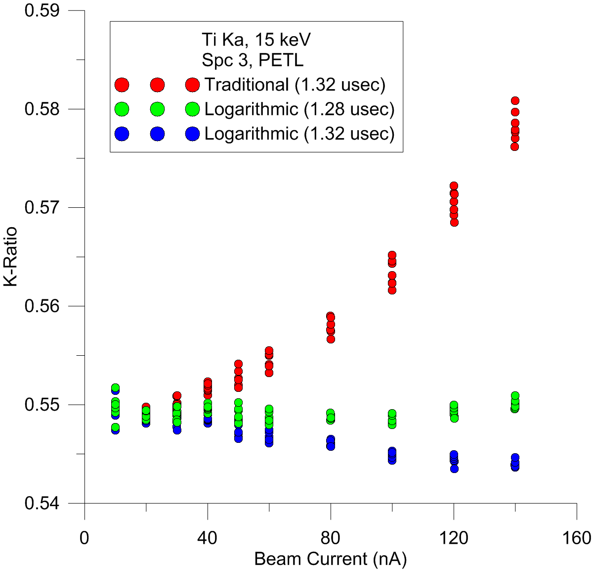
Clearly, if we want to acquire high speed quant maps or measure major, minor and trace elements together, it's pretty obvious that the new dead time expressions are going to yield more accurate results.

And if anyone still has concerns about how these the new logarithmic expression performs at low beam currents, simply examine this zoom of the above plot showing results at 10 and 20 nA:


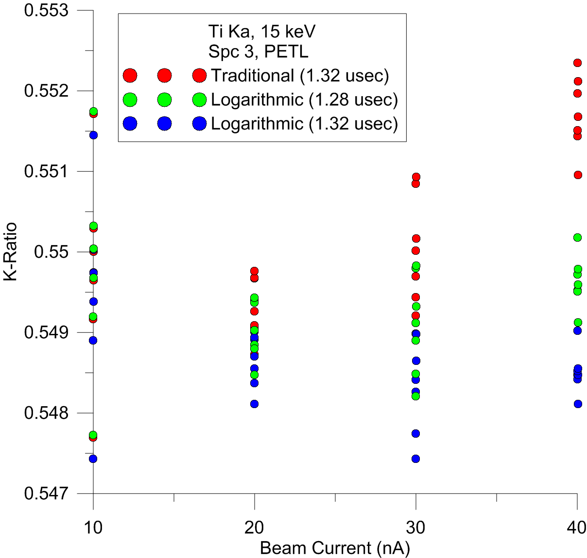
All three are statistically identical at these low beam currents!  And remember, even at these relatively low count rates there are still some non-zero number of multiple photon coincidence events occurring, so we would argue that even at these low count rates, the logarithmic expression is the more accurate expression.

OK, with that out of the way, let's proceed with the promised discussion regarding SG's comments on the factors contributing towards dead time effects in WDS spectrometers, because there is no doubt that several factors are involved in these dead time effects, both in the detector itself and the electronics.

But however we measure these dead time effects by counting photons, they are all combined in our measurements, so the difficulty is in separating out these effects.  But the good news is that these various effects may not all occur in the same count rate regimes.

For example, we now know from Monte Carlo modeling that at even relatively low count rates, that multiple photon coincidence events are already starting to occur. As seen in the above plot starting around 30 to 40 nA (>50K to 100K cps), on some large area Bragg crystals.

As the data reveals, the traditional dead time expression does not properly deal with these events, so that is the rationale for the multiple term expressions and finally the new logarithmic expression. So by using this new log expression we are able to achieve normal quantitative accuracy up to count rates of 300K to 400K cps (up to 140 nA in the first plot). That's approximately 10 times the count rates that we would normally limit ourselves to for quantitative work!

As for nomenclature I resist the term "pulse pileup" for WDS spectrometers because (and I discussed this with Nicholas Ritchie at NIST), to me the term implies a stoppage of the counting system as seen in EDS spectrometers.

However, in WDS spectometers we correct the dead time in software, so what we are attempting to predict are the photon coincidence events, regardless of whether they are single photon coincidence or multiple photon coincidence. And as these events are 100% due to probabilistic parameters (i.e., count rate and dead time), we merely have to anticipate this mathematically, hence the logarithmic expression.

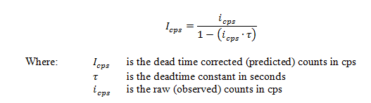
To remind everyone, here is the traditional dead time expression which only accounts for single photon coincidence:


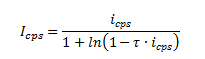
And here is the new logarithmic expression which accounts for single and multiple photon coincidences:


Now, what about even higher count rates, say above 400K cps?  Well that is where I think SG's concerns with hardware pulse processing start to make a significant difference. And I believe we can start to see these "paralyzing" (or whatever we want to call them) effects at count rates over 400K cps (above 140 nA!) as shown here, first by plotting with the traditional dead time expression:


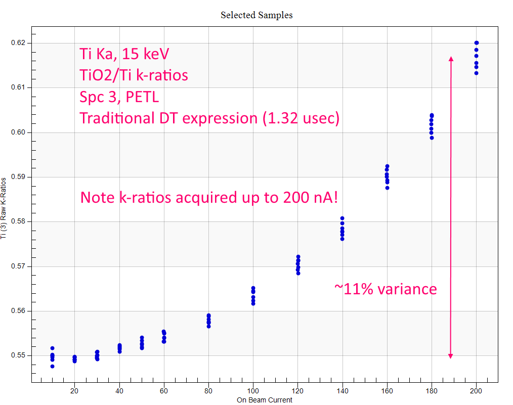
Pretty miserable accuracy starting at around 40 to 60 nA.  Now the same data up to 200 nA, but using the new logarithmic expression:


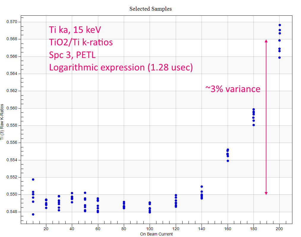
Much better obviously, but also under correcting starting about 160 nA of beam current which corresponds to a predicted count rate on Ti metal of around 450K cps!   :o

So yeah, the logarithmic expression starts to fail at these extremely high count rates starting around 500K cps, but that's a problem we will leave to others, as we suspect these effects will be hardware (JEOL vs. Cameca) specific.

Next we'll discuss some of the other types of instrument calibration information we can obtain from these constant k-ratio data sets.
« Last Edit: August 16, 2022, 10:56:56 AM by Probeman »
The only stupid question is the one not asked!

Probeman

  • Emeritus
  • *****
  • Posts: 2831
  • Never sleeps...
    • John Donovan
Re: New method for calibration of dead times (and picoammeter)
« Reply #67 on: August 17, 2022, 12:49:07 PM »
So once we have fit our dead time to yield constant k-ratios over a large range of range count rates (beam currents), we can now perform high accuracy quantitative analysis from 5 or 10 nA to several hundred nA depending on our crystal intensities and our spectrometer dead times.

Because as we can all agree, we should obtain the same k-ratios (within statistics of course) at all count rates (beam currents). And we can also agree that due to hardware/electronic limitations (as SEM Geologist has correctly pointed out) our accuracy may be limited at count rates that exceed 300K or so cps. And we can see that in the 200 nA plots above when using Ti ka on a large PET crystal when we exceed 400K cps.

But now we can perform additional tests using this same constant k-ratio data set that we used to check our dead time constants, for example we can test our picoammeter linearity.

You will remember the plot we showed previously after we adjusted our dead time constant to 1.28 usec to obtain a constant k-ratio up to 400K cps:


We could further adjust our dead time to flatten this plot at the highest beam current even more, but if we examine the Y axis values, we are clearly within a standard deviation or so.

Now remember, this above plot is using both the primary *and* secondary standards measured at the same beam currents. So both standards at 10 nA, both at 20 nA, both at 40 nA, and so on. And we do this to "null out" any inaccuracy of our picoammeter.

Well, to test our picoammeter linearity we simply utilize a primary standard from a *single* beam current measurement and then plot our secondary standards from *all* of our beam current measurements as seen here:


Well that is interesting, as we see a (very) small discontinuity around 20 to 40 nA in the k-ratios on Anette's JEOL instrument when using a single primary standard. This is probably due to some (very) small picoammeter non-linearity, because after all, we are now depending on the picoammeter to extrapolate from our single primary standard measured at one beam current, to all the secondary standards measured at various beam currents!

In Probe for EPMA this picoammeter linearity is an easy test to perform using the constant k-ratio data set, as we simply use the string selection control in the Analyze! window to select all the primary standards and disable them all, then simply select one of these primary standards (at one of the beam currents) and enable that one primary standard, and then from the Output | Output XY plots for Standards and Unknown dialog, we calculate the secondary standards for all the beam currents, in this case using beam current for the X axis and the k-ratio for the Y axis.

Stray tuned for further instrument calibration tests that can performed using this simple constant k-ratio data set.
« Last Edit: August 17, 2022, 09:32:55 PM by Probeman »
The only stupid question is the one not asked!

Probeman

  • Emeritus
  • *****
  • Posts: 2831
  • Never sleeps...
    • John Donovan
Re: New method for calibration of dead times (and picoammeter)
« Reply #68 on: August 19, 2022, 12:28:11 PM »
And now we come to the third (and to my mind, the elephant in the room) aspect in the use of these constant k-ratios, as originally described by John Fournelle and myself.

We've already described how we can use the constant k-ratio method (pairs of k-ratios measured at multiple beam currents) to adjust our dead time constant to obtain a constant k-ratio over a large range of count rates (beam currents) from zero to several hundred thousand (300K to 400K) cps, as we should expect from our spectrometers (since the lowest count rate k-ratios, should be the least affected by dead time effects).  Note that by measuring both the primary and secondary standards at the *same* beam current, we "null out" any non-linearity in our picoammeter.

Next we've described how on can check for our picoammeter linearity by utilizing from the same data set a single primary standard measured at one beam current and plot our secondary standard k-ratios (from the range of beam currents) to test the beam current extrapolation, and therefore linearity of the picoammeter system.

Finally we come to the third option using this same constant k-ratio data set, and that is the simultaneous k-ratio test.  Now in the past we might have only measured these k-ratios on each of our spectrometers (using the same emission line) at a single beam current as described decades ago by Paul Carpenter and John Armstrong.  But our constant k-ratio data set (if measured on all spectrometers using say the Ti Ka line on LIF and PET and the Si Ka line on PET and TAP), already contains these measurements, so let's just plot them up as seen here:


Immediately we can see that two of these spectrometers (form Anette von der Handt's JEOL instrument at UBC), are very much in agreement, but spectrometer 2 is off by some 4% relative.  This is not an uncommon occurrence (as I have the same effect on my spectrometer 3 of my old Cameca instrument).  Please note that when I first measured these simultaneous k-ratios when my instrument was new, they were all within a percent or two as seen here:

https://probesoftware.com/smf/index.php?topic=369.msg1948#msg1948

but it is concerning in a new instrument.  Have you checked your own instrument?  Here were the results I made during my instrument acceptance testing (see section 13.3.9):

https://epmalab.uoregon.edu/reports/Additional%20Specifications%20New.pdf

Note that spectrometer 3 was slightly more problematic than the other spectrometers even back then...

But it should cause us much concern, because how can we begin to compare our consensus k-ratios from one instrument to another, if we can't even get our own spectrometers to agree with each other on the same instrument?

 :(

If you want to get a nice overview of all three of these constant k-ratio tests, start a few posts above beginning here:

https://probesoftware.com/smf/index.php?topic=1466.msg11100#msg11100
« Last Edit: August 19, 2022, 12:32:07 PM by Probeman »
The only stupid question is the one not asked!

sem-geologist

  • Professor
  • ****
  • Posts: 301
Re: New method for calibration of dead times (and picoammeter)
« Reply #69 on: August 19, 2022, 03:38:05 PM »
Are you sure your sample is perpendicular to the beam? I see something similar like that on our SX100 too. But I am sure that somehow the holder is not perfectly perpendicular to the beam, when compared with newer SXFiveFE. Also recent replacement of BSE detector on SX100 made me aware that it (actualy the metal cover plate) can affect the efficiency of counting at different spectrometer range.

BTW, where is that cold-finger or other cryo system mounted? maybe it is affecting (shadowing) part of x-rays. Large crystals are in particular edgy on shadowing effects as our bitter experiene with newer BSE had shown. Gathering huge number of k-ratios is not in vain - indeed it will be so helpful in identifying some deeply hiden problems with some annonimiously behaving spectrometers! Lets don't stop, but move on!
« Last Edit: August 19, 2022, 03:54:05 PM by sem-geologist »

Probeman

  • Emeritus
  • *****
  • Posts: 2831
  • Never sleeps...
    • John Donovan
Re: New method for calibration of dead times (and picoammeter)
« Reply #70 on: August 20, 2022, 09:46:31 AM »
Are you sure your sample is perpendicular to the beam? I see something similar like that on our SX100 too. But I am sure that somehow the holder is not perfectly perpendicular to the beam, when compared with newer SXFiveFE. Also recent replacement of BSE detector on SX100 made me aware that it (actualy the metal cover plate) can affect the efficiency of counting at different spectrometer range.

As we have discussed there are several mechanical issues which might explain ones spectrometers producing different k-ratios. 

Some relate to sample tilt as you say. Which is why we should if possible measure our constant k-ratios on all of our spectrometers, and include (as Aurelien mentioned in the consensus k-ratio procedure) measuring these k-ratios at several stage positions several millimeters apart in order to calculate a sample tilt.  Probe for EPMA reports sample tilt automatically when using mounts that have three fiducial markings.

The k-ratios above were acquired on Anette's instrument so I cannot say, but I doubt very much that she could have tilted the sample enough to produce a 4% difference in intensity!

The other mechanical issues can be spectrometer alignment or even asymmetrical diffraction of the Bragg crystals resulting in a difference in the effective takeoff angle.  Even more concerning is spectrometer to column positioning due to manufacturing mistakes, as Caltech discovered on one of their instruments many years ago.

On this JEOL 733 instrument Paul Carpenter and John Armstrong found that the so-called "hot" Bragg crystals provided by JEOL were not diffracting symmetrically, resulting in significant differences in their simultaneous k-ratio testing. 

After that had been sorted out by replacing those crystals with "normal" intensity crystals, they found there was still significant differences in the simultaneous k-ratios which they eventually they tracked down to the column being mechanically displaced from the center of the instrument, enough to cause different k-ratios on  some spectrometers.

This was the *last* JEOL 733 delivered as JEOL had already started shipping the 8900.  How many of those older instruments also had the electron column mechanically off-center?  What about your instrument?  There is only one way to find out!    ;D

Measure your constant k-ratios on all your spectrometers (over a range of beam currents) and see if your:

1.  dead times are properly calibrated

2. your picoammeter is linear

3. you get the same k-ratios within statistics on all spectrometers


BTW, where is that cold-finger or other cryo system mounted? maybe it is affecting (shadowing) part of x-rays. Large crystals are in particular edgy on shadowing effects as our bitter experiene with newer BSE had shown. Gathering huge number of k-ratios is not in vain - indeed it will be so helpful in identifying some deeply hiden problems with some annonimiously behaving spectrometers! Lets don't stop, but move on!

I don't know about Anette's instrument, but on our SX100 we see the same sorts of differences in one spectrometer and we have no cold finger. We use a chilled baffle over the pump:

https://probesoftware.com/smf/index.php?topic=646.msg3823#msg3823

But that's certainly something worth checking if your simultaneous k-ratios do not agree and you have a cold finger in your instrument.
The only stupid question is the one not asked!

sem-geologist

  • Professor
  • ****
  • Posts: 301
Re: New method for calibration of dead times (and picoammeter)
« Reply #71 on: August 21, 2022, 10:45:44 AM »
One more real life experience which would make k-ratio biased. It is noise increase in the detector-preamplifier circuit. I had discovered a month ago we have such problems on some spectrometers. On Cameca instruments it is very easy to test it. Set Gain to 4095, while beam is blanked, and look to ratemeter. It should get sporadic jumps at blue level (very few counts per second) from cosmic rays (yes spectrometer is able to be hit by those  :o without a problem). If there is 10-1000cps there is potential problem. If it is high pressure spectrometer that is not so important, but if it is low pressure spectrometer - the problem grows in severity. We have some noise getting in at such gain on few spectrometers on SX100 and SXFiveFE, there in most of cases it dissapears with gain reduced to 2000-3000. However one of spectrometers produces not 1000cps, but 100000cps when having gain at 2500. After inspection of signal with osciloscope I had found that it have much higher noise than other signals of other spectrometers - after I had opened the metal casing of there preamplifier is placed I found out that one of HV capacitors is cracked and that is an obvious noise source. Cracking of these disc capacitors probably does not take a day and I guess such crack could creep making that noise to increase slowly in many years.

Why noise is important? Because if noise is leaks into counting (and triggers the counting) then dead-time corrected k-ratios will be biased, as such noise would effect the detection more at low count rates than at high count rates. I think older Jeol (is new too?) models would be effected even more buy such hardware aging as background noise is passed to PHA. In Case of Cameca instruments it is much easier to identify such problem.
« Last Edit: August 22, 2022, 02:53:15 AM by sem-geologist »

Probeman

  • Emeritus
  • *****
  • Posts: 2831
  • Never sleeps...
    • John Donovan
Re: New method for calibration of dead times (and picoammeter)
« Reply #72 on: August 22, 2022, 08:39:43 AM »
This reminds me of one of the tests that John Armstrong performed on one of the first JEOL 8530 instruments at Carnegie Geophysical.  I think he called it the "beam off test", because he would test the PHA electronics when the beam was turned off, and what he found was that he was seeing x-ray counts with no electron beam!

These counting artifacts were eventually tracked down to JEOL changing suppliers for some chips in the spectrometer pre-amp which were noisier than the original specification and therefore causing these spurious counts.
The only stupid question is the one not asked!

Probeman

  • Emeritus
  • *****
  • Posts: 2831
  • Never sleeps...
    • John Donovan
Re: New method for calibration of dead times (and picoammeter)
« Reply #73 on: August 22, 2022, 09:39:56 AM »
Parametric Constant:

a. A constant in an equation that varies in other equations of the same general form, especially such a constant in the equation of a curve or surface that can be varied to represent a family of curves or surfaces

At this point I think it would be helpful to discuss what we mean when we refer to the dead time as a "constant".

Because if there is one thing we can be sure of, it's that the dead time is not very constant since it can obviously vary from one spectrometer to another!  More importantly it can even vary for a specific detector as it becomes contaminated or as the electronic components age over time. I've even seen the dead time constant change after replacing a P-10 bottle!  P-10 composition?

In addition, we might suspect that the dead time could vary as a function of x-ray emission energy or perhaps the bias voltage on the detector, though these possible effects are still under investigation by some of us.  I hope some of you readers will join in these investigations.

So this should not be surprising to us since the dead time performance of these WDS systems include many separate effects in both the detector and counting electronics (and possibly even satellite line production!), all which are convolved together under the heading of the "dead time constant".

But it should also be clear that when we speak of a dead time "constant", what we really mean is a dead time "parametric constant", because it obviously depends on how we fit the intensity data and more importantly, what expression we utilize to fit the intensity data. Here is an example of the venerable dead time calculation spreadsheet from Paul Carpenter plotting up some intensities (observed intensity vs. beam current):


The question then becomes: which dead time "constant" should we utilize in our data corrections?  That is, should we be fitting the lowest intensities, the highest intensities, all the intensities? How then are we calling this thing a "constant"?   :D

Here is another thought: when we attempt to measure some characteristic on our instruments, what instrumental conditions do we utilize for measuring that specific characteristic? In other words how do we optimize the instrument to get the best measurement?

For an example by analogy, when characterizing trace elements, we might increase our beam energy to create a larger interaction volume containing more atoms, and we will probably also increase of beam current, and probably also our counting time, as all three changes in conditions will improve our sensitivity for that characterization.  But we also want to minimize other instrumental conditions which might add uncertainty/inaccuracy to our trace characterization.  So we might for example utilize a higher resolution Bragg crystal to avoid spectral interferences, or perhaps Bragg crystal with a higher sin theta position to avoid curvature of the background.  Or we could utilize better equations for correction of these spectral interferences and curved backgrounds!    8)

Similarly, that is also what we should be doing when characterizing our dead time "constants"!  So to begin with we should optimize these dead time characterizations by utilizing conditions which create the largest dead time effects (high count rates) and we should also apply better equations which fit our intensity data with the best accuracy (over a large range of beam currents/count rates).

So if we are attempting to characterize our dead time "constant" with the greatest accuracy, what conditions (and equations) should we utilize for our instrument?  First of all we should remove the picoammeter from our measurements, because we don't want to include any non-linearity to these measurements since we are depending on differences in count rates at different beam currents.  The traditional dead time calibration fails in this regard. However, both the Heinrich (1966) ratio method and the new constant k-ratio method exclude picoammeter non-linearity from the calculation by design, so that is good.

But should we be utilizing our lowest count rates to calculate our dead time constants? Remember, the lowest count rates not only provide the lowest sensitivity (worse counting statistics), but also contain the *smallest* dead time effects!  Why would we ever want to characterize a parameter when it is the smallest effect it can possibly be?  Wouldn't we want to characterize this parameter when its effects are most easily observed, that is at high count rates?    :o

But then we need to make sure that our (mathematical) model for this (dead time) parameter properly describes these dead time effects at low and high count rates!  Hence the need for a better expression of photon coincidence as described in this topic.

Next let's discuss sensitivity in our dead time calibrations...
The only stupid question is the one not asked!

Probeman

  • Emeritus
  • *****
  • Posts: 2831
  • Never sleeps...
    • John Donovan
Re: New method for calibration of dead times (and picoammeter)
« Reply #74 on: August 23, 2022, 10:45:52 AM »
Before I continue writing about sensitivity, I just want to emphasize an aspect of the constant k-ratio method that I think is a bit under appreciated by some.

And that is that for the purposes of determining the dead time constant (and/or testing picoammeter linearity and/or simultaneous k-ratio testing), the constant k-ratio method does not need to be performed on samples of known composition. Whatever the k-ratio is observed to be (at a low count rate using a high precision logarithmic or multiple term expression), that is all we require for these internal instrumental calibrations.

The two materials could be standards or even unknowns. The only requirement is that they contain significantly different concentrations of an element, and be homogeneous and relatively beam stable over a range of beam currents.

In fact, they can be coated differently (e.g., oxidized or not), and we could even skip performing a background correction for that matter!  We only care about the ratio of the intensities, measured over a range of beam currents/count rates!  :o   All we really require is a significant difference in the count rates between the two materials and then we can adjust the dead time constant (again using a high precision expression) until the regression line of the k-ratios is close to a slope of zero!

 8)

Of course when reporting consensus k-ratios to be compared with other labs using well characterized global standards, we absolutely must perform careful background corrections and be sure that our instrument's electron accelerating energies, effective take off angles and dead time constants are well calibrated!
« Last Edit: August 23, 2022, 11:12:42 AM by Probeman »
The only stupid question is the one not asked!