Modeling Inclusions/Particles Embedded in a Matrix

[John Donovan]

Another case is the modeling of particles or inclusions embedded in a matrix of another composition. The attached screen shot shows a 5 um Cu particle embedded in an Al matrix (the <n>mic_sphere.geo geometry files are all 50% buried hemisphere geometries).  Remember that one needs to be logged in to see attachments!

The barely visible Al Ka signal is due to secondary fluorescence from the Cu Ka and continuum x-rays generated in the Cu inclusion.

Note that the minimum electron/photon energies (circled in red) should be the same for both materials and set to a value below the ionization energy of the lowest energy emission line of interest.

Note on using the *sphere geometry files:
Note that when using the hemisphere geometry files, make sure that the X beam position shown here is properly set. The default for the straight line boundary geometry (couple.geo), is 10 um (1E-3 cm) to the right into the beam incident material.

If it is desired to place the beam in the exact center of the inclusion, set the X distance to zero as shown here:

[John Donovan]

Calculating k-ratios from Penepma generated intensities:

It is probably worth explaining how to calculate k-ratios from Penepma photon intensity calculations. Generally we want to utilize elemental k-ratios, therefore in addition to calculating the photon intensities for our unknown sample at the specific conditions and geometry desired, we will also need to calculate the pure element intensities for the element emission of interest at the same sample conditions, though generally for a bulk geometry.

Therefore at least two Penepma calculation models must be run, one for the unknown and one for the standard. Of course each element in the unknown calculation that will be converted to a k-ratio needs a (generally bulk) standard calculated also. In the above example of a Cu particle in an Al matrix that means three input files: one for the unknown inclusion in the matrix, one for the pure bulk Al and one for the pure bulk Cu.

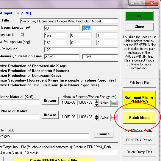
The easiest way to do this is to utilize the "batch" mode of the Penepma GUI, by first generating the two input files from the Create PENEPMA Material and Input Files window which is accessed in the Standard.exe program from the Analytical | PENEPMA (Monte Carlo) Calculations menu.

Once all Penepma input files have been generated, simply click the Batch Mode button as seen here:



and then select the input files you want to run from the input file list. The basic calculation parameters are displayed as each input file is selected (use <ctrl> click for multiple selections), and when all input files have been selected, Browse to (and create if necessary) a folder to store your calculation results in as shown here:



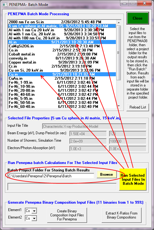
Then simply click the Run Select Input Files In Batch Mode button.  The program will confirm the required calculation time and folder to save to (each calculation and output files will be automatically saved to a separate sub folder), and then simply click OK to start the calculation.

Extracting the intensities for k-ratio calculations:

Once all the Monte-Carlo calculations are complete, one browses to the batch output folders shown here:



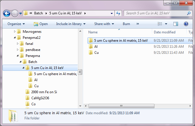
Now locate the pe-intens-01.dat file in each folder and copy or note the transition intensity for each line that you desire to calculate k-ratio values for. The most common transitions are listed here:

K L3       ' (Ka) (see table 6.2 in Penelope-2006-NEA-pdf)
K M3       ' (Kb)
L3 M5      ' (La)
L2 M4      ' (Lb)
M5 N7      ' (Ma)
M4 N6      ' (Mb)


An example from one of the three output files is shown here, specifically the unknown sample (Cu hemisphere in Al):

#  Results from PENEPMA. Output from photon detector #  1
 #
 #  Angular intervals : theta_1 = 4.500000E+01,  theta_2 = 5.500000E+01
 #                        phi_1 = 0.000000E+00,    phi_2 = 3.600000E+02
 #
 #  Intensities of characteristic lines. All in 1/(sr*electron).
 #    P = primary photons (from electron interactions);
 #    C = flourescence from characteristic x rays;
 #    B = flourescence from bremsstrahlung quanta;
 #   TF = C+B, total fluorescence;
 #  unc = statistical uncertainty (3 sigma).
 #
 # IZ S0 S1  E (eV)      P            unc       C            unc       B            unc       TF           unc       T            unc
   29 L1 M3  1.0228E+03  1.954288E-06 2.68E-07  0.000000E+00 0.00E+00  2.207194E-09 2.50E-09  2.207194E-09 2.50E-09  1.956495E-06 2.68E-07
   29 L1 M2  1.0228E+03  1.162781E-06 2.06E-07  0.000000E+00 0.00E+00  1.576567E-09 2.12E-09  1.576567E-09 2.12E-09  1.164358E-06 2.06E-07
   29 L1 M4  1.0927E+03  1.223980E-08 2.12E-08  0.000000E+00 0.00E+00  0.000000E+00 0.00E+00  0.000000E+00 0.00E+00  1.223980E-08 2.12E-08
   29 L1 M5  1.0930E+03  4.079933E-09 1.22E-08  0.000000E+00 0.00E+00  0.000000E+00 0.00E+00  0.000000E+00 0.00E+00  4.079933E-09 1.22E-08
   13  K L2  1.4863E+03  2.744367E-09 2.93E-09  3.577180E-08 1.11E-08  9.888903E-08 1.65E-08  1.346608E-07 2.76E-08  1.374052E-07 2.01E-08
   13  K L3  1.4867E+03  8.534549E-09 5.16E-09  6.731252E-08 1.52E-08  1.939424E-07 2.31E-08  2.612549E-07 3.84E-08  2.697895E-07 2.82E-08
   13  K M2  1.5576E+03  0.000000E+00 0.00E+00  0.000000E+00 0.00E+00  6.028973E-10 1.28E-09  6.028973E-10 1.28E-09  6.028973E-10 1.28E-09
   13  K M3  1.5576E+03  0.000000E+00 0.00E+00  7.692860E-10 1.63E-09  9.043460E-10 1.57E-09  1.673632E-09 3.20E-09  1.673632E-09 2.26E-09
   29  K L2  8.0278E+03  1.026919E-05 6.15E-07  0.000000E+00 0.00E+00  2.809442E-07 2.86E-08  2.809442E-07 2.86E-08  1.055014E-05 6.16E-07
   29  K L3  8.0478E+03  2.028543E-05 8.64E-07  0.000000E+00 0.00E+00  5.410777E-07 4.01E-08  5.410777E-07 4.01E-08  2.082651E-05 8.66E-07
   29  K M2  8.9054E+03  1.244380E-06 2.13E-07  0.000000E+00 0.00E+00  2.680164E-08 8.82E-09  2.680164E-08 8.82E-09  1.271181E-06 2.14E-07
   29  K M3  8.9054E+03  2.570358E-06 3.07E-07  0.000000E+00 0.00E+00  6.747706E-08 1.39E-08  6.747706E-08 1.39E-08  2.637835E-06 3.08E-07
   29  K M4  8.9771E+03  4.079933E-09 1.22E-08  0.000000E+00 0.00E+00  0.000000E+00 0.00E+00  0.000000E+00 0.00E+00  4.079933E-09 1.22E-08

If we are interested in the Al Ka and Cu Ka emissions we simply note the "K L3" photon intensity values in the T column (total intensity and its uncertainty (unc) just to the right).

Remembering that the <K ratio intensity> = <Unk intensity> / <Std intensity>, we save these unknown photon intensity values to be the numerators for our k-ratios. Note that in the case of the K emissions we may also include the Kb emission intensity to improve our precision, by adding in the contribution of the Kb "K M3" transition, since all K emissions are emitted from the same edge.

Now, obtain the same corresponding "K L3" photon intensity values from the pure (bulk) Al and pure (bulk) Cu folder pe-intens-01.dat files and insert the the corresponding intensity values in the denominator of our k-ratio equation to calculate the elemental k-ratio for Al Ka and Cu Ka in our unknown sample relative to the pure elements.

Houston: we have k-ratios!

[Mike Spilde]

Hi John,
I'm trying to figure out how to analyze small (micrometer-sized) inclusions of pyrrhotite (FeS) in pentlandite (Fe,Ni)8S9. I wonder if you might provide a more detailed tutorial on PENEPMA using the geometry files? Can we apply the calculations in CalcZAF to correct the Ni-fluorescence on Fe in the same way that we would for a boundary fluorescence problem?

Thanks,
Mike
 

[Probeman]

Hi Mike,
I assume you're trying to figure out if the FeS inclusions have a trace amount of Ni in them?

If so, you only have to worry about continuum fluorescence because the Fe and S characteristic x-rays will not fluorescence any Ni atoms in the matrix material.

But let's see what effect it will have by running Standard.exe and using the Penfluor/Fanal calculation to start as described in painful detail here:

http://probesoftware.com/smf/index.php?topic=58.0

So, let's run at 15 keV (as opposed to 20 keV) to minimize the interaction volume which we normally might want to for trace Ni!  We can note first however that by using this calculation:

http://probesoftware.com/smf/index.php?topic=86.0

at 15 keV the Ni interaction volume in FeS is just under 1 um so we are close but OK:



So, assigning FeS as our beam incident material and FeNi (50:50 by weight) as our boundary material (because I haven't calculated a Pentlandite yet!) we obtain the following Penfluor/Fanal result:



This is a worst case because there's more Ni in Fe-Ni than in Pentlandite, but it tells you you could very well have a problem analyzing trace Ni in FeS adjacent to Pentlandite.

If you want to calculate the effect for Pentlandite as a boundary material (and you will have to calculate Pentlandite if you want to make the boundary correction in CalcZAF or even if you do it by hand!), it will take about 10 hours to calculate the PAR file and the process is described here:

http://probesoftware.com/smf/index.php?topic=58.msg214#msg214

I hope this helps.

[John Donovan]

I'm trying to figure out how to analyze small (micrometer-sized) inclusions of pyrrhotite (FeS) in pentlandite (Fe,Ni)8S9. I wonder if you might provide a more detailed tutorial on PENEPMA using the geometry files? Can we apply the calculations in CalcZAF to correct the Ni-fluorescence on Fe in the same way that we would for a boundary fluorescence problem?

Hi Mike,
I re-read your question and realize I should add the following points:

1. The Penfluor/Fanal secondary boundary fluorescence modeling in Standard.exe will only work for vertical boundaries.

2. However, ignoring "tertiary effects", one can assume that a lamellae with a width twice that of the vertical boundary calculation distance will have an artifact intensity roughly twice as large. However, that assumption is based on the point equidistant from the two boundaries.

3. For an inclusion the geometric effect is even larger, obviously somewhere between 2 and 4 times the effect from a single vertical boundary. I'm working with a mathematician to try and "transform" these intensity profiles into different geometries such as a hemisphere.

4. In the meantime your best bet is to run the full Penepma 2012 from Standard.exe and select one of the "[hemi]sphere" geometry files as described above.  A little more work, but you'll get the right answer!

[Sheri Singerling]

Hi John,

Thanks for this post; it's been very useful! I am looking at Fe,Ni-metal inclusions (~1 to 2 microns in diameter) in sulfides in a group of meteorites. Can we do the k ratio corrections in CALCZAF when we use a sphere geometry? Or is that function in CALCZAF (as you described it in "Topic: Nasty Boundary Fluorescence Analytical Situations") only limited to a boundary geometry? If that's the case, I take it we just manually calculate the k ratios as you describe above using the "pe-intens-01.dat" files? Thanks!

[Probeman]

Funny you should ask that, I've been working with a mathematician to see if we can "re-normalize" the Fanal calculation output to include other geometries such as particles. For example, if your analysis position is equi-distant from two lamellae, then your total SF contribution is roughly twice that of a single boundary (ignoring third order effects). For a sphere (or hemisphere), it will be between 3 and 4 times the single boundary intensity. We want to transform the single boundary intensity into other geometrical intensities but have not completed this yet...

As for modifying the FORTRAN MC code, unfortunately, the Fanal code was written with a dependence on mirror symmetry and cannot be easily modified according to Cesc Salvat.

So the answer at the present time is no.  But as you say, you can still run the full Penepma GUI with particle geometries, which I should mention has recently been improved so be sure to update.

[Sheri Singerling]

Ok, I finally have my data from the microprobe and the k-ratios from the PENEPMA simulations. How do I actually go about correcting my probe data with these SF k-ratios since CalcZAF isn't an option for the sphere geometry? I haven't been able to find anything describing that process so if you could point me in the general direction, that would be fantastic. Thanks!

[Probeman]

Ok, I finally have my data from the microprobe and the k-ratios from the PENEPMA simulations. How do I actually go about correcting my probe data with these SF k-ratios since CalcZAF isn't an option for the sphere geometry? I haven't been able to find anything describing that process so if you could point me in the general direction, that would be fantastic. Thanks!

The advantage of doing it in CalcZAF, is that *if* there is a large change in the concentrations due to the SF correction, this could affect the matrix correction, especially for low energy x-ray lines. In CalcZAF, the SF correction is iterated and therefore automatically handles this change in composition.

But usually the SF correction is small enough that this can be ignored, and in that case a simple subtraction of the boundary contribution in wt.% (material B), from the measured concentration will be sufficient.  In the kratio2.dat file, it is this column:



One way to check this is to run CalcZAF with the uncorrected concentrations and again with the corrected concentrations and see how different the matrix correction term (ZAFCOR) is between the two for each emitting element.  If it is less than a percent or so, I wouldn't worry, though you could apply it.

For reference please use the paper attached below.

Wait!  I just realized that you used Penepma, not Fanal for this modeling so the Fanal output screen shot doesn't help you!

The problem is that Penepma doesn't separate the beam incident contribution from the SF boundary contribution. So if you have some of the element present in the beam incident material, you'll have the intensity of that added in with the SF intensity.

What you'll need to do is calculate your material with a boundary (as you've already done), then calculate the same material *without* a boundary and subtract the appropriate line intensities from each other.

Does that make sense?  Then you can apply that k-ratio intensity difference to your measurements by converting them to concentrations (just multiply the k-ratio by the matrix correction for this material).

[Sheri Singerling]

Alright, I'll try that out asap! One more question. This applies to the pe-intens-01.dat files and how you setup the files for the standards. You mentioned how we must have PENEPMA calculate intensities for the standards in addition to our beam incident-boundary materials. I just want to make absolutely sure I've done those simulations correctly because I've gotten very odd k ratios by dividing the I_unk by I_std. I've attached screenshots of the parameters I used for each .IN file (Setups.jpg). I'm mostly concerned that I haven't set up the standard .IN files correctly. The standard setups are labeled "Fe", "Ni", and "S". My beam incident material setup is labeled "metal". I've also attached the pe-intens-01 files for each as well (Outputs.jpg). As you can see, dividing the unknown intensity by the standard intensity (I focused on the Ka intensities) from these numbers gives you K ratios of 1 for S and Ni and 0.99927 for Fe. Any clues as to what I may have done wrong with my setup? Thanks again!

Edit by John: I note that 500 seconds is a very short simulation time and that because of this your uncertainties on the "T" values for the K L3 (Ka) are around 5 to 10%. But it's good to "work out the bugs" as they say on short runs such as this.

Also, I would run the the standards using the normal "Optimize Production of Characteristic X-rays" (first) option.  The SF option might work for a single material, but I have never run it this way, so try and see if that helps.

I'll try some simulations myself overnight and let you know what I find.

Note also that the standard can be a compound, but then you'll have to calculate the std K-factor for which you'll need the pure element std calculated anyway!

[John Donovan]

I ran your compositions as a simple boundary in Fanal just as a "sanity check", and as you can see:



and depending on the size of the inclusion there will be a significant enhancement of the inclusion from secondary (continuum) fluorescence. Why is it continuum fluorescence only? Because Fe and S characteristic x-rays cannot fluoresce the Fe K edge.

Note that the opposite can occur when the matrix is low Z such as epoxy as John Fournelle has described in the links here:

http://probesoftware.com/smf/index.php?topic=58.msg209#msg209

[John Donovan]

Sheri,
It just occured to me that you might be doing too much work!

All you need to calculate (to begin with) is a pure Fe std, your inclusion geometry and a bulk version of your inclusion composition, so

1. Fe
2. Fe90Ni10 bulk
3. Fe90Ni10 inclusion in FeS2.

Then ratio both Fe90Ni10 Fe Ka (K L3) intensities to the pure Fe Ka (K L3) std intensity. That intensity ratio difference is the SF effect with and without the geometric effects and it will vary with the beam position (the default position X = 0, Y = 0 is the center of the inclusion, but remember it's in cm).

Since you are using a pure Fe std, the k-ratios you obtain are elemental k-ratios and therefore represent the percent effect when multiplied by 100.

Does that help?

[Sheri Singerling]

Thanks for helping me with this John! What about S though? When I ran the Fanal for a boundary condition with Fe90Ni10 and FeS (pyrrhotite not pyrite; I just use pyrite as my standard for my microprobe analyses so that's why it's popped up in some of this discussion), it looks like I'm getting some SF. I've attached the resulting plot. Note that the density for my Fe90Ni10 is wrong. Not quite sure how I did that, but I ran my Fe90Ni10 and FeS2 just to compare to what you got above, and they are similar. So I'm thinking the general problem of SF of S will still exist even with the correct density of Fe90Ni10. I'll have to run another .PAR file if I want to fix that, but for the non-Fanal simulations, I'm using my .MAT files which I've fixed the density for.

Additionally, I ran into some major problems with the pe-intens-01 files yesterday and this morning. What I've found is that the pe-intens-01 files are basically overwriting one another. For example, for my pyrite pe-intens-01 file, I don't have any data listed for S. There is only data for Fe and Ni. I then compared this to my Fe90Ni10 pe-intens-01 file, which also only has Fe and Ni (as it should I suppose), and found that they are exactly the same. The time stamps for the files are also identical meaning it was the same file. Any ideas what this is about? I tried deleting any old batch files and any .IN files and rerunning everything, but the problem still persists. Exiting out of Standard.exe didn't solve the problem either. Thanks again!

[John Donovan]

Hi Sheri,
Yes density matters when distance is a factor.

Yes, I didn't model sulfur but it looks like it is getting fluoresced by Fe and Ni Ka.

The main Penepma window is designed for creating input files and they can be run one at a time there, but as you say, the Run Input File in PENEPMA button will overwrite your previous work.  To avoid this simply use the "Batch Mode" button as described here:

http://probesoftware.com/smf/index.php?topic=59.msg221;topicseen#msg221

and the files will all automatically get saved to the specified folder including the input, geo and mat files like this as they are completed:

[Sheri Singerling]

I ran it using the batch mode but still had the files being duplicated. There seems to be something with the order that the files are run which determines which ones are duplicated. For example, I initially ran the following .IN files:
- one for my Fe90Ni10 inclusion surrounded by FeS (using the 1 micron sphere .geo file) -> metal.IN
- one for my Fe standard (using the bulk file) -> Fe.IN
- one for my Ni standard (using the bulk file) -> Ni.IN
- one for my S standard (using the bulk file) -> S.IN
- one for my pure, bulk Fe90Ni10 (using the bulk file) -> pureMetal.IN
PENEPMA ran them in the following order (based on the time stamp on the folders in the batch folder): Fe -> metal -> Ni -> pureMetal -> S.
The pe-intens-01 files that were the same were the metal and the Ni files, and then the pureMetal and the S files. The Fe pe-intens-01 had a time stamp from yesterday so maybe it is a duplicate of the last simulation I ran yesterday. Any ideas? Maybe I should reinstall the whole penepma file.