Nasty Boundary Fluorescence Analytical Situations

[John Donovan]

This thread is for those of you that have come across some problematic secondary boundary fluorescence situations, either through modeling or measurement.  In fact it would be nice to compare the modeling with any measurements you all have performed.

To start off I thought I would mention the simple point that if the boundary fluorescence is extremely large as in the Co-Cu default example in Standard.exe (Analytical | PENFLUOR/FANAL (Monte-Carlo) Calculations menu) and seen in the first attachment below, one can often ascertain that there is a significant issue without even running a model since the totals will often be obviously too high if the boundary fluorescence effect is large enough. 

This is often seen in the case of a traverse over a boundary and noting that the totals at the boundary are usually significantly higher than 100%.  Clearly these cases usually involve both a pure boundary fluorescence effect where most electrons come to rest in the beam incident material, but as the beam approaches the boundary there will be some degree of electron excitation of both phases on each side of the boundary and this will yield incorrect matrix corrections usually also resulting in high totals. And of course combinations of both effects depending on the exact beam position relative to the boundary and the physics details.

It should be also noted that in less common cases where the self-fluorescence of one phase is very large, one can also observe a low total in the measurement when the fluoresced element is *not* present in the boundary material. This has been noted by John Fournelle and Xavier Llovet and published in this paper on inclusions in a non-fluorescing matrix (e.g. epoxy):

http://www.geology.wisc.edu/~johnf/g777/777Penelope/Llovet_Valovirta_et_2000.pdf

John also has a nice presentation on this:

http://epmalab.uoregon.edu/Workshop2/Fournelle-Penelope.pdf

But the point I'm attempting to make here is that in many cases where the secondary fluorescence artifact is much smaller the effect is less obvious in the totals, especially when a trace or even minor element is being measured as in a diffusion profile. In these cases only MC modeling will reveal the magnitude of the error.

The second attachment below demonstrates a 100 PPM artifact at over 500 um distance from the boundary. This boundary artifact was observed at Oak Ridge National lab and was a cause for some concern at the time. Note the log scale in the concentration axis.

[Gseward]

Hi John,
I've run the Penepma secondary boundary fluorescence GUI in Standard.exe for a number analytical problems, but would you mind posting an example for all of us showing the steps for doing this calculation, both for modeling the situation and also for correcting measured intensity data for these artifacts, maybe a simple system such as Ti Ka in quartz next to rutile or Ti Ka in zircon next to rutile? 

Cheers,

Gareth

[John Donovan]

Excellent idea!

I'll do this in several parts to make it manageable.

We will make use of Standard.exe and CalcZAF.exe for these calculations.  Both programs are available for free by downloading the CalcZAF.msi installer from here:

http://probesoftware.com/Technical.html

Note that the Penepma12.ZIP (Penepma 2012 file and data set) is now included with the CalcZAF.msi installer and will be installed automatically to your UserData folder when CalcZAF or Standard are run the first time if it is not already installed.

The first section using Standard.exe will describe creating the material (*.MAT) and parameter (*.PAR) files for the boundary modeling (and matrix modeling as well if the beam incident and boundary phases are the same composition!)

The second section (again using Standard.exe) will describe using the PAR files for boundary (and bulk matrix modeling) to determine if a problematic situation is present by extracting k-ratios based on the stage coordinates of the analysis positions and the boundary distance and orientation.

The third section will focus on correcting intensity measurements for boundary artifacts if the sample k-ratios are imported into CalcZAF along with the stage positions. The CalcZAF correction implementation that will be shown below is for demonstration and testing purposes, and is limited to corrections for one element at a time.

Finally please note that the k-ratio intensities are reported in % in order that they can be displayed together with the concentrations in wt. %.

The Probe for EPMA software will provide a full automatic correction for boundary artifacts for multiple elements once it is fully implemented in our main EPMA software later this year.

Stay tuned...

[John Donovan]

First section: Creation of material and parameter files.

The first step in modeling boundary artifacts is to check if the material phases you plan to model, already have PAR files calculated for them. 

This is because once a PAR file is calculated for a specific material (~10 hours each for typical precision), one can utilize this PAR file to extract k-ratio intensities for *any x-ray emission line*, at *any keV* (between 5 and 50 keV) and at *any distance* from the boundary. So the PAR file calculation is time consuming but provides many re-uses for different analytical situations.

Therefore, before beginning the creation of material and parameter files for a phase, first check that the phase under investigation hasn't already been calculated. Note that all pure elements are already calculated along with approximately 200 common phases. Additional phases are continually being calculated and uploaded. A thread discussing newly calculated compounds which can be downloaded is found here:

http://probesoftware.com/smf/index.php?topic=13.0

After starting Standard.exe and clicking on the Analytical | Penepma (Secondary Fluorescence Profile) Calculations menu to open the Calculate Penepma 2012 Fluorescence Couple Profiles window (see attached screen shot of the full window at the very bottom for reference), the first step then is to check the Penfluor folder for existing PAR files by clicking on the Browse button as shown here:



Be sure to check the Compound sub folder as shown here as most compounds will be stored there at first (pure elements will be found in the Pure subfolder):



We will need three materials for each boundary fluorescence calculation. The beam incident material, the boundary material and the standard for the k-ratio calculation. If the boundary calculation is for modeling purposes only, then one should generally use a pure element as the standard since then the program can calculate additional information which may be saved to an Excel spreadsheet for further study.

However, if the calculation will be used for correction of measured k-ratio intensities, one must use the same standard as used for the measured k-ratio intensities on the instrument.

If all three phases are already calculated as PAR files, one can skip to the second section. Otherwise proceed by either selecting a material from the current standard database (making sure that the density value in the text field is correct) as shown here:



and click the Create Material A From List button, or enter the density of the phase (density is important since the intensities are reported in linear distances) and click the Create Material A From Formula button. Three sets of buttons are provided in case one needs to calculate all three materials.

These material calculations only take 30 to 60 seconds for each material and the newly created .MAT files are loaded automatically in the PAR file calculation area below.

When the necessary material files are ready to be calculated as PAR files one can click any of the buttons circled here to calculate all three or any one:



Again, each PAR file calculation takes approximately 10 hours each.  The next section will describe how to use the PAR files for extracting k-ratio intensities to model boundary artifacts or matrix corrections.

[John Donovan]

Second Section: Extraction of K-ratio Intensities From PAR Files.

Continuing our modeling of Ti Ka in SiO2 adjacent to TiO2, we turn our attention to the Calculate Secondary Fluorescence Profiles For The Specified Element and Xray section of the window, and make sure that the Material A (beam incident) is specified as SiO2, Material B (boundary) is specified as TiO2, and Material B Std (primary std) is either the pure element (Ti) or the standard actually used in the measurement on the instrument (e.g., TiO2) as seen here:



Next make sure the correct element and x-ray line is selected, in this case Ti Ka, and that the correct take off angle and beam energy is specified (e.g., 15 keV).

Finally specify the total distance the modeling should cover in microns and the number of points to calculate. The default values of 50 um and 50 points (i.e., 1 um per point) is usually sufficient but can be modified as desired. Note again that because the intensities are reported in linear distances (um), the correct material densities are very important for accuracy.

One can also opt that the quite extensive output file kratio2.dat also be saved to an Excel spreadsheet, but all other output files are automatically saved. For example,  For example, this calculation would be saved to a folder named 15_SiO2_TiO2_Ti_22_1 in the C:\UserData\Penepma12\fanal\couple folder. Where 15 is the keV, SiO2 is the beam incident material, TiO2 is the boundary material, Ti is the standard and 22_1 refers to the emitting element and line (1 = Ka, 2 = Kb, 3 = La, etc).

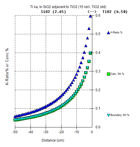
For more information on the data types saved please refer to the Probe for EPMA Reference manual by hitting F1 as shown in the attached screenshot at the end of the post.  Remember that one needs to be logged in to see attachments!

When ready click the Run Fanal (generate k-ratio file for couple boundary) button and after 20 to 30 seconds the data will be displayed in the graph area as shown here:



Note that the material densities and other essential information is displayed in the graph title. The critical information are the k-ratio intensity points. These intensities are utilized in the correction procedure that will be described in the third section.

Several other concentration related data types are plotted as follows:

Boundary Wt.%:  This is the concentration of the boundary intensity artifact that is contributed from the boundary material *only*. However since there is no Ti in this SiO2 material, the "Calc Wt.% and the "Boundary Wt.%" plot on top of each other.

In situations where the beam incident material contains a non-zero concentration of the emitted element, the  "Calc Wt.% and the "Boundary Wt.%" will plot differently.

Calc Wt.%:  The concentration that should be reported if the software was properly noting the fact that the Ti concentration is *not* actually present in the beam incident material (SiO2), but instead is in the boundary material (TiO2). However, since the "spurious" concentration of Ti in the SiO2 is relatively small, the matrix correction of Ti ka in pure SiO2 is approximately 1.202 while the matrix correction for Ti ka in SiO2 with 0.4 wt.% Ti is approximately 1.201. Therefore the former calculation in pure SiO2 is reported as the "Calc. Wt.%, while the latter calculation in SiO2 with a minor amount of Ti is reported as the "Meas. Wt.%".

Meas. Wt.%:  As stated above, the "Meas. Wt.%" is the concentration that would be reported by your microprobe software since it incorrectly assumes that the Ti Ka is being emitted in an SiO2 matrix. Of course this reported value is "not even wrong" since the Ti Ka is actually being emitted from the TiO2 boundary phase!

As an aside, the default example of Co ka measured in Cu adjacent to Co, shows an example of how a large artifact affects the assumed matrix correction as seen here:



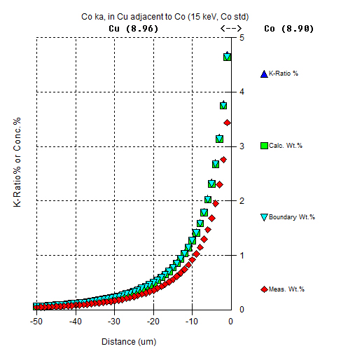
It is interesting to note in the above Co Ka example, that since the beam incident, boundary materials and standard are pure elements, the k-ratio intensities (in %) and Calc. Wt.% concentrations are the same.

Finally it should be mentioned again that since the correction of this artifact utilizes the modeled k-ratio intensities, it is critically important that the correct standard be modeled for use in the third section in the subsequent post. But the pure element is sufficient for general modeling and in fact allows the program to output additional matrix information since the standard k-factor does not need to be calculated.

An example of the Ti Ka in SiO2 adjacent to TiO2 using TiO2 as a standard as opposed to pure Ti is shown here:



Note that the reported concentrations are same but that the k-ratio intensities are quite different due to the use of the TiO2 as the standard instead of Ti.

[John Donovan]

Third Section: Correction of Secondary Boundary Fluorescence Artifacts

This section will describe how to correct for SF boundary artifacts using CalcZAF. CalcZAF will only correct for one element artifact at a time, which is sufficient for demonstration and testing, but by the end of this year (2013) we hope to have a multi-element SF boundary artifact correction implemented in Probe for EPMA. This PFE implementation will use the same dialog as below but will also have the ability to store and recall all specified parameters automatically for all elements for your probe run.

Begin by first generating a model of the analytical situation in Standard.exe where you suspect a secondary boundary fluorescence exists as described in the previous replies above.

As a slight aside, note that these artifacts usually cause an increase in the apparent concentration of the measured element, but in certain situations where the sample under investigation is self-fluorescing and the boundary phase (or matrix in the case of an inclusion geometry) does *not* contain that fluoresced element, one may see a *decrease* in apparent concentration as discussed in the first post of this thread. Another example of a "negative" SF artifact can be seen in certain boundary situations as shown here:



So the first step is to decide if there is a significant secondary boundary fluorescence artifact worth correcting using Standard.exe.

In any event, once you have modeled your specific analytical situation in Standard.exe with the appropriate materials, keV and element/x-ray parameters and preferably out to a distance from the boundary so that the artifact intensity is close to zero, you can proceed to the correction of this boundary fluorescence using CalcZAF.

From the Analytical | Correct Secondary Fluorescence Boundary Effects menu in CalcZAF you will see this window when it is first opened:



You will note that there are two methods for SF correction, but only the first (top) option is currently available. Start by browsing to the folder where your SF model was automatically saved to. As previously mentioned, the file we are looking for (kratios.dat) will be in a folder named for the analytical conditions.

For example, for Ti Ka in SiO2 adjacent to TiO2 using a Ti standard at 15 keV, the kratios.dat file would be saved to a folder named 15_SiO2_TiO2_Ti_22_1 in the C:\UserData\Penepma12\fanal\couple folder. Where 15 is the keV, SiO2 is the beam incident material, TiO2 is the boundary material, Ti is the standard and 22_1 refers to the emitting element and line (1 = Ka, 2 = Kb, 3 = La, etc).



The program will confirm the essential parameters of the selected kratios.dat file as shown here:



Now enter the boundary coordinates that will apply to the correction. One may manually specify the boundary by typing in a fixed distance, stage coordinates and angle, or two stage coordinates, but the easiest method if you are using Probe for EPMA, is to import a stage calibrated SE or BSE image acquired from PFE using the Browse For Image button as shown here:



If you imported an image, now you simply draw the boundary using the mouse. You can draw the boundary as many times as you like until you feel it is correct:



Now you will need to import a data file containing the measured k-ratios. The easiest way to do this is to export the analysis intensities from Probe for EPMA using the Output | Save CalcZAF Format menu (I'll be adding another right click method to the Analyze! window for exporting specific samples to the CalcZAF format soon).

The format of the CalcZAF import file is documented in detail in the User's Reference but the basic structure is fairly obvious:

3,2,15,40., "SiO2 adjacent to TiO2 (Elemental K-ratios)", -25,  0., 0.
1,"si","",0.0,"","",0.0
"ti","ka",1,1,0,0.,.00075,0.0
"si","",1,2,0,0.,.0,0.0

The above example is for a single data point, but there are sample data sets with a full Ti ka SiO2 traverse for both JEOL and Cameca stages in the C:\UserData\CalcZAFDATData (or your default user data) directory named:

Wark-Watson Exper. Data (CalcZAF format)_Cameca.dat
Wark-Watson Exper. Data (CalcZAF format)_JEOL.dat

For this data importation one can use the CalcZAF app File | Open CalcZAF Input Data File menu and process the data points one at a time using the Calculate button to see the analysis *without* the SF correction, or using the Calculate Current Composition button to see the the analysis *with* the SF correction.

Use the Load Next Dataset From Input File button to advance through the import file one data point at a time. See the two attachments at the end of this post for examples of both with and without the SF correction for the first data point in the example files.

Finally one can also process a complete data set using the Open Input File and Calculate/Export All button as shown here:



Pretty neat!

Edit 02/04/14 : right click method for CalcZAF output has been implemented in the Analyze! window sample list for output of selected samples.

[Ravi]

Hi John,
Thanks for your posts on this very interesting topic. I will try those corrections/steps and see how it goes.
Meanwhile, I am attaching a BSE image showing the Qti data I measured sometime back on a Qtz_Ti couple (the grains glued next to each other and polished).

The picture (attached below) describes it all.

[Ravi]

Thanks John for the nice plot and comparison with Wark & Watson's data!

[jon_wade]

Hi all

I hope John doesn't mind me chipping in, but I thought I would post an example or two of where secondary fluorescence can give rise to 'erroneous' data and how tools such as PENEPMA and FANAL, embedded within P4W, can  offer a  handle on the SF contribution.

The first one is the high precision analysis of trace Ca within the olivine.  This is the basis for the olivine-CPX geobarometer, however, the fine-grained nature of the rocks often leads to problems of secondary fluorescence masking the true Ca content of the olivines.  To show how good the simulations are, I recreated the work of Adams and Bishop (1986) who performed a very detailed EPMA study to 'back out' the SF contribution.  I did this by recreating a synthetic ol-cpx couple in PENEPMA (see below).  The nice thing  is that these codes allow you to use both the actual, measured, compositions , and also change the geometry of both the sample (i.e. buried sphere, crystal etc) and the detector (i.e. take-off angle, size etc).

Adams and Bishop, through an exceptional series of EPMA analyses concluded that at 15um from a planar CPX:Ol boundary, their Ca-free olivine would exhibit ~220ppm of Ca, arising purely from SF of the Ca in in the neighbouring CPX.
My  PENEPMA simulations gave ~230ppm at the same distance using the same compositions (and a lot less effort!). 

I did this using PENEPMA, but FANAL gives a similar result in a lot less time, and better still converts k-ratio to concentration for you.  This allows us to  correct the real EPMA data by simply subtracting the SF concentration, derived from the simulation, from the real EPMA data collected at the same distance from the phase boundary.

Edit by John: Jon, I cherish your "chipping in"! I particularly like the comparison of the two detector geometries. Please continue chipping in!

[jon_wade]

Ok, so I now believe the simulation codes work (and are an order of magnitude or two easy to perform than the equivalent probe analyses) what can I do with them?

One obvious application is analysing high pressure experiments.  A inevitable consequence of performing very high pressure experiments is that there's a corresponding decrease in sample size - and very high pressure experiments obviously lead to very small samples! 

Element partitioning studies are often anchored upon the analysis of trace components within a phase, surrounded by a host where the element of interest is a major component. Furthermore, high-pressure experiments often compound the analytical difficulty, as phases are often small in size and incapable of being physically separated and mounted individually. In such a case there is always the potential that the assumption of a chemically homogeneous matrix (required for the matrix correction routine) is not valid and/or neighbouring phases contribute to the analysis.  This is especially true of very high pressure samples generated in the Diamond Anvil Cell (DAC), where samples are often so small as to be extremely difficult to handle.

To explore the potential influence of SF, I simulated a 22.4GPa DAC experiment of (Bouhifd and Jephcoat, 2003). This work investigated the conditions of planetary core formation, and in particular the partitioning behaviour of Ni and Co between Ni-rich metal and Ni-poor silicate phases.  As an aside, theres often been a bit of a 'mismatch' between the Ni partitioning data generated using multi-anvil high pressure devices and DACs, and the suspicion has been that this is either an experimental or analytical 'artefact' of some kind.

I used this work simply because it helpfully (and unusually) includes both the elemental data of both phases present, together with a micrograph of the experiment from which it was obtained and the location of where the analyses were made. This means that its possible to perform a realistic simulation with PENEPMA and assess the SF contribution on the Ni analyses of the silicate (if any), arising from the near-by Ni rich metal.

I simulated an simplistic version of the experiment using either a half - or 2/3 buried ball of metal, in a matrix of silicate of the correct composition (but Ni free) and simulated analyses of the silicate at various distances away from the metal (again, see below).

The result is that, at the analytical conditions the authors used,  the simulations show that if the analyses were performed ~ 5um from the phase boundaries, the reported Ni concentrations need to be reduced by ~25%.  A not insignificant amount, but more importantly, this brings the results back into line with those generated by multi anvil high pressure devices (which typically generate larger sample volumes at these pressures).

I hope this has been of some interest; I'm a fully paid-up member of the PENEPMA/FANAL fan club, and find their application to a variety of problems (FIB-sections, thin films etc etc) really useful, and if anyone wants any more info, feel free to post, message or email me.

All the best

Jon


[edit] the figure captions in the attached files - B refers to a cartoon of the SEM picture of the run product , C&D to the results.  figure A was going to be a the original micrograph from the paper, but the household picture editor informed me of copyright rules just in time!

[John Donovan]

Finally fixed the data cursor when the K-Ratio% plot is in log10 scale as seen here:

[John Donovan]

This is the proper thread for Penfluor/Fanal calculations...

I decided to ZIP up all the low energy PAR files that I have already done and make them available here:

http://probesoftware.com/download/PAR_lessthan1000eV.zip

The ones labeled 500eV are good for oxygen Ka and fluorine Ka, the 200eV ones are good for carbon Ka and nitrogen Ka.

Note that these 200 eV PAR files could also be used for oxygen and fluorine emission modeling, but the 200 eV files will have somewhat poorer statistics for the oxygen and fluorine primary (electron beam) excitation intensities, so better to use PAR files that are calculated to an energy no lower than the emitted energy (which will always be less than the edge energy).

Remember, these PAR files currently can only be utilized in a "couple" geometry, that is, a straight line vertical boundary by Fanal. For (hemi)sphere geometries, the intensities must be calculated using the full Penepma method, which is the subject of this topic:

http://probesoftware.com/smf/index.php?topic=59.0

[Probeman]

I've been doing some interesting comparisons between couple and hemisphere geometries for C Ka in Fe99Ni adjacent to pure carbon for Ed Vicenzi as seen here:

http://probesoftware.com/smf/index.php?topic=59.msg1384#msg1384

One of the tests I ran using Penepma was a zero distance boundary measurement where the beam would impact exactly at the boundary, ideally producing a k-ratio close to 0.5 (neglecting the small C ka SF issue).

The results from 50K seconds of calculations at 20 keV are here:

0 um distance intensity = 9.6009E-05   +/- 4.95E-06
Bulk Carbon intensity = 1.8832E-04    +/- 2.73E-06

K-ratio = 0.5098

Of course we expect a slightly higher than 0.5 k-ratio due to a small amount of C ka SF and the extra 0.0098 we see here is similar to the Penpema value at 1 um distance plotted in the above link.

PS: the 200eV PAR files ZIP used for such calculations has been updated here:

http://probesoftware.com/download/PAR_lessthan1000eV.zip

[John Donovan]

This plot relates to the discussion in the modeling inclusions topic here:

http://probesoftware.com/smf/index.php?topic=59.msg1384#msg1384

But I am posting it here to discuss the intensity differences between the full Monte-Carlo calculated by Penepma and the Penfluor MC and Fanal SF analytical modeling of couple boundaries. Here is a plot of Penepma and Penfluor/Fanal calculating the secondary fluorescence effect on C ka in Fe99Ni1 adjacent to pure carbon.



Note that the extra C Ka intensity seen in the Penepma intensity calculations at distances less than 2 microns from the boundary are due to electron scattering across the couple boundary. This effect will be much larger for the inclusion geometry.

Note also that the Penfluor/Fanal intensity output is in K-ratio% and so should be divided by 100 to compare to the Penepma k-ratios obtained by dividing intensities from the pe-intens-01.dat files.

By the way, if you'd like to run the Penfluor/Fanal calculation with Fe/Ni adjacent to epoxy as opposed to pure carbon, the 200 eV PAR file (HCNO_200eV.par) is attached below.

[Probeman]

I finally got around to creating an epoxy PAR file (Epon 828 which apparently contains ~0.3% of Cl) and I ran it next to a mineral glass to see what level of secondary fluorescence one might obtain and at 15 keV this is what you see:



Obviously this could be a concern for determining trace levels of Cl in glass adjacent to epoxy, e.g., mounted tephra specimens.

The epoxy PAR file will soon in the normal distribution but I've attached it below for now.

Note also that the full Penepma GUI in Standard.exe now supports multiple detector geometries:

0. Annular (0 to 360 degrees)
1. North
2. East
3. South
4. West



Each "cardinal" direction detector is +/- 20 degrees from 0, 90, 180 and 270 degrees around the specimen. The detectors all are centered on the takeoff angle +/- 5 degrees (e.g., for 40 degrees take off they are 35 to 45 degrees from the specimen surface or 45 to 55 degrees from the perpendicular).