Continuing from the post above...
Now let's correct for these SF effects. Start by selecting the sample(s) in the Analyze! window sample list and then click the Boundary Corrections button in the Analyze! window. The Secondary Fluorescence Correction from Boundary Phase dialog will open as seen here:

Note that the above steps can be performed in any order but all need to be completed before the SF corrections can be performed. In the above example, we simply selected an image from our saved images, then we clicked the Define Boundary Method button to define the boundary to open the Secondary Fluorescence Boundary Correction Parameters dialog as seen here:

In the above example, we clicked the Specify Graphical Boundary option and then using the mouse, we drew a boundary on the image as shown (one can also specify the boundary geometry using stage positions if an image is not available). The boundary was drawn partially in the gap between the phases because the physics we modeled is not exactly correct because we assume no gap in PENFLUOR/FANAL physics calculations. Note that normally you will not have a gap between your phases so this issue can be ignored for now, but there are ways of dealing with a gap between phases that can be discussed later.
Note also that we oriented this synthetic boundary in the instrument so that the boundary was pointing directly at the WDS spectrometer (Fe ka) making the trace measurement. For EDS spectrometers, this is not necessary, but until we implement a Bragg defocus geometry correction in Probe for EPMA (see
https://academic.oup.com/mam/article-abstract/24/6/604/6901481 by Ben Buse et al. 2018) it is best to avoid Bragg defocus effects by orienting the sample relative to the spectrometer. However, for boundary distances less than 10 or 15 um these Bragg defocus effects will be minimal. If two trace elements need to be measured/corrected together, then spectrometers that are diametrically opposed to each other should be selected with the phase boundary pointing at both spectrometers.
Ok, let's proceed by now browsing for our modeled boundary fluorescence k-ratios.dat file as seen here:
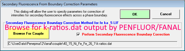
If the correct file was selected, the k-ratios as a function of boundary distance will be loaded as shown previously above. Note that on the right side we can see the Mat A, Mat B and Mat B std materials utilized in the PENFLUOR/FANAL calculations. Now we just click OK and click the Analyze button again:
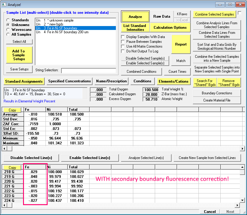
Wasn't that easy!

Ok, well it's better than doing it manually by hand...
To provide some additional details, these calculated k-ratios are subtracted from the measured k-ratios during the matrix correction procedures, so even if significant SF boundary corrections are performed, the calculation of the other elements in the modified matrix will be properly accounted for (in this regard this is similar to the quantitative spectral interference correction in PFE)
Though it should be mentioned that if the change in composition from the SF boundary correction is not large one can simply subtract the calculated concentrations in Excel or otherwise. But the advantage of doing it in PFE is that the process is completely documented and fully quantitative.
Now one last note: the SF boundary calculation in PENFLUOR/FANAL assumes a vertical infinite boundary interface, which is not always the case of course with our samples. We are also investigating the possibility of performing a geometrical correction to deal with hemispherical geometries for example, but in the meantime one can perform these boundary calculations the PENEPMA code using the Standard application as described here:
https://probesoftware.com/smf/index.php?topic=59.0One would need to model each distance from the boundary so that will take a while, but one can use the Batch Mode button in the PENEPMA GUI to make it easy:
https://probesoftware.com/smf/index.php?topic=151.0Then one would need to extract the k-ratios from each distance and create your own k-ratios.dat file similar to what is produced by PENFLUOR/FANAL (and the Fanal.txt file as well) and place it in an appropriately named folder.
Anyway, this is a new feature, so we'll be interested to hear from you all on using it for your own specific examples.


 Please keep your software updated for best results!