Author Topic: Improving Time Dependent Intensity (TDI) Corrections (Read 13283 times)

Probeman · « **on:** November 18, 2013, 12:44:24 PM »

I'm opening this topic with the intent to create a place to discuss improving the Time Dependent Intensity (TDI) correction in Probe for EPMA for beam sensitive sample acquisition. If you want to ask questions or comment on the existing TDI correction please use this topic link here:

http://probesoftware.com/smf/index.php?topic=11.0

The reason for this is that although the TDI correction is PFE works well well for almost all beam sensitive samples (both "volatile" and "grow-in" artifacts as documented by many investigators, such as Stuart Kearns, http://www.geology.wisc.edu/~johnf/g777/AmMin/Humphreys_2006.pdf, and George Morgan, http://www.geology.wisc.edu/~johnf/g777/AmMin/MorganLondon2005.pdf), there are still some situations requiring an even more robust TDI correction due to the limited size of the sample (requiring a more focused beam), or element sensitivity (requiring a higher beam current).

And let's be honest, if we could run these samples at cryogenic temperatures as suggested by Stuart Kearns we could use our existing TDI methods just fine, but almost no one (not even Stuart anymore!), has an EPMA instrument with a cryogenic stage, (Electronprobe Microanalysis of Volcanic Glass at Cryogenic Temperatures (2002) S.L. Kearns,N. Steen and E. Erlund, Microscopy and Microanalysis 8 (Supple 2), 1562-1563CD), so we need a robust software solution that works even under less than ideal conditions.

Please feel free to chime in with your questions, observations and comments. This topic is for all researchers working with beam sensitive materials in EPMA.

Probeman · « **Reply #1 on:** November 18, 2013, 02:01:49 PM »

Ok, let's start by reviewing what we can do with the Time Dependent Intensity (TDI) correction in Probe for EPMA, which I believe is the best method currently available. By the way, to give credit where credit is due, Paul Carpenter suggested we use the term Time Dependent Intensity, rightly I would say, because then we are not assuming physics we don't fully understand (sample heating, sub-surface charging, ion migration, changes in the matrix absorption due to ion migration, etc.).

Here we see a large but otherwise typical TDI correction (note most of the examples we will discuss will be from Na intensities, but the PFE TDI correction applies equally well to all elements that undergo changes in intensity as a function of beam exposure, e.g., K, Si, Al, F, P, etc.):

The above example has a Na TDI correction percent of almost 80%. Not too bad for losing almost half one's Na intensity as seen here:

Un 17 Withers-N5, Results in Elemental Weight Percents ELEM: Na K Cl Ba F Ti Fe Mn Ca Si Al Mg O H TYPE: ANAL ANAL ANAL ANAL ANAL ANAL ANAL ANAL ANAL ANAL ANAL ANAL ANAL SPEC BGDS: MAN LIN LIN LIN LIN LOW MAN LIN MAN MAN MAN MAN EXP TIME: 60.00 20.00 10.00 20.00 40.00 10.00 40.00 10.00 20.00 20.00 20.00 60.00 120.00 BEAM: 9.98 9.98 9.98 9.98 9.98 9.98 9.98 9.98 9.98 9.98 9.98 9.98 9.98 ELEM: Na K Cl Ba F Ti Fe Mn Ca Si Al Mg O H SUM 574 2.780 3.536 .205 .030 .086 .108 3.136 .060 .162 32.680 5.404 .012 50.078 .665 98.943 575 3.072 3.557 .207 .017 .084 .124 3.120 .079 .148 32.990 5.365 .007 49.939 .594 99.303 576 2.846 3.314 .180 .032 .100 .137 3.131 .083 .129 32.914 5.316 .000 49.919 .624 98.727 577 2.925 3.550 .258 .041 .111 .098 3.165 .058 .118 32.858 5.437 -.001 49.985 .621 99.224 578 3.011 3.502 .258 -.014 .083 .072 3.173 .081 .116 32.715 5.364 .009 49.812 .626 98.810 579 3.043 3.561 .239 -.079 .070 .124 3.191 .083 .130 32.812 5.428 .006 50.012 .623 99.244 580 2.842 3.531 .223 .016 .089 .101 3.125 .055 .132 32.799 5.335 -.001 49.969 .644 98.859 581 3.179 3.459 .248 -.019 .121 .118 3.100 .050 .152 33.024 5.362 .006 50.053 .605 99.455 582 2.924 3.505 .164 -.025 .080 .134 3.197 .051 .120 33.124 5.375 .009 49.790 .562 99.009 583 2.890 3.436 .218 -.062 .033 .147 3.165 .031 .143 32.919 5.388 .003 49.908 .609 98.830 584 2.952 3.381 .213 .004 .033 .124 3.124 .064 .133 33.068 5.325 .004 49.852 .588 98.865 585 2.699 3.608 .191 .029 .071 .121 3.150 .061 .161 33.000 5.380 .006 50.223 .641 99.341 AVER: 2.930 3.495 .217 -.003 .080 .117 3.148 .063 .137 32.909 5.373 .005 49.962 .617 99.051 SDEV: .133 .084 .030 .038 .026 .020 .030 .016 .016 .139 .038 .004 .122 .028 .248 SERR: .038 .024 .009 .011 .008 .006 .009 .005 .005 .040 .011 .001 .035 .008 %RSD: 4.54 2.40 13.87-1523.47 33.10 17.21 .97 25.48 11.67 .42 .70 80.01 .24 4.47 STDS: 336 374 285 835 835 22 395 25 358 162 336 12 12 0 STKF: .0735 .1132 .0601 .7430 .1715 .5546 .6779 .7341 .1693 .2018 .1331 .4737 .2328 .0000 STCT: 2447.9 2423.7 839.3 8520.6 2398.7 6097.6 14136.8 13590.2 2247.6 34290.6 23223.7 24410.3 8335.9 .0 UNKF: .0154 .0303 .0017 .0000 .0002 .0010 .0261 .0005 .0012 .2688 .0412 .0000 .2315 .0000 UNCT: 513.0 648.1 24.2 -.2 2.7 10.8 545.2 9.5 16.2 45673.8 7190.2 1.7 8290.2 .0 UNBG: 9.9 12.6 5.0 29.0 3.8 5.8 23.4 16.1 4.4 134.1 103.2 15.2 53.7 .0 ZCOR: 1.9017 1.1548 1.2500 1.3725 4.0763 1.1972 1.2041 1.2234 1.1196 1.2241 1.3036 1.4987 2.1582 .0000 KRAW: .2096 .2674 .0289 .0000 .0011 .0018 .0386 .0007 .0072 1.3320 .3096 .0001 .9945 .0000 PKBG: 52.69 52.56 6.39 1.00 1.77 3.03 24.32 1.61 4.71 341.58 70.64 1.11 156.16 .00 INT%: ---- ---- ---- -3.81 ---- -.02 ---- ---- ---- ---- ---- ---- ---- ---- APF: ---- ---- ---- ---- ---- ---- ---- ---- ---- ---- ---- ---- 1.031 ---- TDI%: 79.930 .454 ---- ---- ---- ---- ---- ---- ---- -.870 ---- ---- -3.030 ---- DEV%: 2.7 2.4 ---- ---- ---- ---- ---- ---- ---- .3 ---- ---- .3 ---- TDIF: QUADRA LINEAR ---- ---- ---- ---- ---- ---- ---- LINEAR ---- ---- LINEAR ---- TDIT: 72.58 30.67 ---- ---- ---- ---- ---- ---- ---- 31.00 ---- ---- 129.42 ---- TDII: 522. 660. ---- ---- ---- ---- ---- ---- ---- 45860. ---- ---- 8327. ---- BLNK#: ---- ---- ---- ---- ---- ---- ---- ---- ---- ---- ---- ---- 19 ---- BLNKL: ---- ---- ---- ---- ---- ---- ---- ---- ---- ---- ---- ---- 43.5580 ---- BLNKV: ---- ---- ---- ---- ---- ---- ---- ---- ---- ---- ---- ---- 44.9622 ----

Potassium is much less affected at 0.454 % (not even statistically significant) and silicon and oxygen are minor corrections (-0.87 and -3.03 % respectively, though both statistically significant).

By the way, the above calculation is for water by stoichiometry to measured excess oxygen as first described by Barbara Nash, http://www.geology.wisc.edu/courses/g777/AmMin/Nash.pdf.

Expressed as oxides the results are seen here for this glass made by Tony Withers and water determined by FTIR at 5.06 wt%:

Un 17 Withers-N5, Results in Oxide Weight Percents ELEM: Na2O K2O Cl BaO F TiO2 FeO MnO CaO SiO2 Al2O3 MgO O H2O SUM 574 3.747 4.260 .205 .033 .086 .180 4.034 .078 .227 69.915 10.212 .019 .000 5.947 98.943 575 4.142 4.284 .207 .018 .084 .207 4.014 .102 .207 70.578 10.138 .011 .000 5.311 99.303 576 3.836 3.992 .180 .036 .100 .229 4.028 .108 .180 70.415 10.045 .001 .000 5.576 98.727 577 3.943 4.276 .258 .046 .111 .164 4.072 .075 .165 70.295 10.274 -.001 .000 5.548 99.224 578 4.059 4.219 .258 -.015 .083 .120 4.082 .105 .163 69.989 10.135 .015 .000 5.597 98.810 579 4.102 4.290 .239 -.088 .070 .207 4.105 .107 .182 70.196 10.257 .009 .000 5.567 99.244 580 3.831 4.253 .223 .018 .089 .169 4.020 .070 .184 70.168 10.080 -.002 .000 5.755 98.859 581 4.285 4.166 .248 -.021 .121 .196 3.988 .064 .213 70.650 10.131 .009 .000 5.405 99.455 582 3.942 4.222 .164 -.028 .080 .224 4.114 .065 .168 70.863 10.155 .014 .000 5.026 99.009 583 3.895 4.139 .218 -.069 .033 .246 4.072 .040 .200 70.426 10.181 .006 .000 5.443 98.830 584 3.980 4.073 .213 .004 .033 .207 4.020 .083 .186 70.744 10.061 .006 .000 5.256 98.865 585 3.638 4.346 .191 .033 .071 .202 4.052 .079 .225 70.599 10.165 .010 .000 5.730 99.341 AVER: 3.950 4.210 .217 -.003 .080 .196 4.050 .081 .192 70.403 10.153 .008 .000 5.513 99.051 SDEV: .179 .101 .030 .043 .026 .034 .039 .021 .022 .298 .071 .007 .000 .247 .248 SERR: .052 .029 .009 .012 .008 .010 .011 .006 .006 .086 .021 .002 .000 .071 %RSD: 4.54 2.40 13.87-1523.47 33.10 17.21 .97 25.48 11.67 .42 .70 80.01 159.54 4.47 STDS: 336 374 285 835 835 22 395 25 358 162 336 12 12 0

Full details of this method are described here:

http://epmalab.uoregon.edu/reports/Withers%20hydrous%20glass.pdf

Probeman · « **Reply #2 on:** November 18, 2013, 02:53:32 PM »

All this is great, so what's the problem?

Well as mentioned previously, sometimes we have to focus the beam and/or increase the beam current and this can cause a number of additional artifacts. The first I will focus on is the so called "incubation time" described by Stuart Kearns which can be seen in a number of compositions, but the high Na glasses prepared for NIST provides extremely beam sensitive materials that can be useful in these investigations, as we can see here in the low time resolution TDI acquisition on K-0373 NIST glass (10 nA, 10 um):

A higher time resolution TDI acquisition will make this artifact even more obvious:

I suspect that what we are seeing here with this "incubation time" is the warming of the sample by the electron beam. That is to say, ion migration of alkali elements towards the sub surface charge implanted by the electron probe does not start, until the sample spot is heated sufficiently. This hypothesis is further supported by a number of acquisitions where it is observed that it is the first point that almost always shows this "incubation time" effect most strongly. In the previous 10 nA, 20 um beam TDI acquisition it can be seen by displaying all the data points for the sample as seen here:

This can also be confirmed by displaying the x and y stage positions of these analyses as seen here:

Note that with a 10 um beam, the 10 um spaced points are essentially adjacent, and therefore the previous point provides a heating time to eliminate sufficient to reduce the "incubation time". Which brings me to a partial solution for this issue.

Clearly if the "incubation time" is variable due to the proximity of previous TDI acquisitions we will have to be more careful about our selection of points for analysis. But if the "incubation time" is fairly reproducible we could utilize a delay in acquisition after the faraday cup is removed, but before the intensity acquisition begins. Interestingly enough, this feature is already built into Probe for EPMA but intended for another application. Called the "Decontamination Time" it was intended to be used for carbon analysis (Pinard and Richter) to allow time for the native hydrocarbon layer on the sample to be removed prior to the count integration as seen here:

So what's next? Let's examine some other TDI acquisition log slopes more carefully, starting with this acquisition on yet another high Na NIST glass (K-1718) at 10 nA and 10 um, which shows several slopes in exponential space as seen here:

What's a micro analyst to do?

qEd · « **Reply #3 on:** November 19, 2013, 08:35:40 AM »

Oh so back to the problematic issue of slope dermination. The first order approach any salt of the earth spectroscopist would use involves displaying the 1st derivative followed by user interaction by defining the range of time over which the slope is determined.

qEd · « **Reply #4 on:** November 19, 2013, 10:16:53 AM »

Breaking out the slope of the earliest/first time dependency mechanism is the most (or only) critical measurement to make as it directly impacts the magnitide of the signal at t=0 unless you are studying the ongoing physics of e- beam-matter interaction itself.

For the materials I have examined such changes take place over relatively short periods of time secs. Hence the challenge is to collect data at short intervals, at the expense of statistics. Once too much time has passed you are potentially either 1)within another of damage regime, or 2) have integrated over an interval so large the slope of the natural log curve is less accurate.

Probeman · « **Reply #5 on:** November 19, 2013, 02:19:51 PM »

Hi Ed,
I agree completely, especially on the point that we are dealing with several different physical regimes with different time scales, e.g., thermal conductivity vs. ion migration vs. sub surface charge dissapation, but here are my two points (worth one cent each).

1. It is usually better if there is less human subjectivity involved in any analytical procedure. Yes, I could add several user adjustable parameters, but I have found that humans (and I think I can include myself in that group!), have difficulty not adjusting things to the way they want it to be, as opposed to a purely statistical/mathematical decision made by the computer.

So maybe the program should alternately try different fit models until it finds the least average deviation?

What I'm getting at is maybe adding an exponential fit to the existing linear (exponential) and quadratic (hyper-exponential) models, which means in log space we now have a double exponential fit, is worth a try. Such considerations are what this topic is for.

2. The long term (40 or more seconds) TDI acquisition might not only be useful for physics modeling. Maybe it will be possible to back out water vs. hydroxyl based on the slope at different time periods. Yes, I just made that up, but we don't know what we don't know!

Basically I think that I'd like to have the most robust fit available for whatever the data looks like and I agree, it might be that we want to count short TDI intervals to capture the initial intensity at time = 0, but that doesn't mean that we should have to acquire TDI data that way- maybe we have a beam sensitive trace element?

So let's look at where we are on the most beam sensitive material that I have found, the K-1781 NIST glass. Here is an analysis, 10 nA, 10 um *without* any TDI correction:

St 171 Set 9 K-1718 NBS Glass, Results in Elemental Weight Percents SPEC: O TYPE: SPEC AVER: 43.050 SDEV: .000 ELEM: Na Si Ca Fe P BGDS: LIN EXP LIN LIN EXP TIME: 40.00 40.00 40.00 40.00 40.00 BEAM: 10.58 10.58 10.58 10.58 10.58 ELEM: Na Si Ca Fe P SUM 56 7.849 29.765 4.000 11.140 .008 95.813 57 7.696 30.010 3.958 11.078 -.017 95.775 58 8.004 29.527 3.969 11.224 -.029 95.746 59 7.703 29.477 3.985 11.022 .040 95.277 60 7.822 29.776 3.952 11.185 .044 95.829 AVER: 7.815 29.711 3.973 11.130 .009 95.688 SDEV: .126 .215 .020 .081 .033 .232 SERR: .056 .096 .009 .036 .015 %RSD: 1.61 .72 .50 .73 349.44 PUBL: 14.837 28.048 3.574 10.491 n.a. 100.000 %VAR: -47.33 5.93 11.17 6.09 --- DIFF: -7.022 1.663 .399 .639 --- STDS: 336 14 285 162 285 STKF: .0735 .4101 .3596 .0950 .1599 STCT: 76.73 79.39 602.77 66.49 40.15 UNKF: .0382 .2422 .0367 .0945 .0001 UNCT: 39.89 46.89 61.54 66.11 .02 UNBG: .31 .13 1.04 .98 .06 ZCOR: 2.0450 1.2267 1.0819 1.1776 1.4231 KRAW: .5199 .5906 .1021 .9944 .0004 PKBG: 143.98 389.44 60.42 69.66 .50

Only a -50% error! Now the same measurements with the linear (exponential) TDI fit:

St 171 Set 9 K-1718 NBS Glass, Results in Elemental Weight Percents SPEC: O TYPE: SPEC AVER: 43.050 SDEV: .000 ELEM: Na Si Ca Fe P BGDS: LIN EXP LIN LIN EXP TIME: 40.00 40.00 40.00 40.00 40.00 BEAM: 10.58 10.58 10.58 10.58 10.58 ELEM: Na Si Ca Fe P SUM 56 17.153 28.107 3.841 11.115 .008 103.273 57 16.928 26.992 3.739 11.054 -.017 101.746 58 17.702 27.520 3.730 11.198 -.029 103.172 59 16.806 27.754 3.718 10.997 .040 102.365 60 17.048 27.434 3.747 11.160 .044 102.484 AVER: 17.128 27.561 3.755 11.105 .009 102.608 SDEV: .346 .411 .049 .081 .033 .628 SERR: .155 .184 .022 .036 .015 %RSD: 2.02 1.49 1.31 .73 348.95 PUBL: 14.837 28.048 3.574 10.491 n.a. 100.000 %VAR: 15.44 -1.73 5.08 5.85 --- DIFF: 2.291 -.487 .181 .614 --- STDS: 336 14 285 162 285 STKF: .0735 .4101 .3596 .0950 .1599 STCT: 78.13 79.81 605.49 66.49 40.15 UNKF: .0875 .2181 .0348 .0945 .0001 UNCT: 93.06 42.45 58.61 66.11 .02 UNBG: .31 .13 1.04 .98 .06 ZCOR: 1.9564 1.2636 1.0786 1.1749 1.4144 KRAW: 1.1911 .5319 .0968 .9944 .0004 PKBG: 335.08 353.48 57.57 69.66 .50 TDI%: 133.257 -9.459 -4.765 ---- ---- DEV%: 7.1 2.7 2.5 ---- ---- TDIF: LINEAR QUADRA LINEAR ---- ---- TDIT: 94.00 94.00 92.80 ---- ---- TDII: 84.3 42.4 59.5 ---- ----

Now only a +15% error. Next we use the quadratic (hyper-exponential) fit:

St 171 Set 9 K-1718 NBS Glass, Results in Elemental Weight Percents SPEC: O TYPE: SPEC AVER: 43.050 SDEV: .000 ELEM: Na Si Ca Fe P BGDS: LIN EXP LIN LIN EXP TIME: 40.00 40.00 40.00 40.00 40.00 BEAM: 10.58 10.58 10.58 10.58 10.58 ELEM: Na Si Ca Fe P SUM 56 16.267 28.049 3.841 11.117 .008 102.332 57 15.369 26.894 3.739 11.058 -.017 100.093 58 15.942 27.409 3.731 11.203 -.029 101.305 59 15.072 27.641 3.719 11.002 .040 100.523 60 15.408 27.329 3.748 11.164 .044 100.744 AVER: 15.611 27.464 3.756 11.109 .009 100.999 SDEV: .482 .424 .049 .081 .033 .864 SERR: .216 .190 .022 .036 .015 %RSD: 3.09 1.55 1.30 .73 348.95 PUBL: 14.837 28.048 3.574 10.491 n.a. 100.000 %VAR: 5.22 -2.08 5.10 5.89 --- DIFF: .774 -.584 .182 .618 --- STDS: 336 14 285 162 285 STKF: .0735 .4101 .3596 .0950 .1599 STCT: 78.13 79.81 605.49 66.49 40.15 UNKF: .0791 .2181 .0348 .0945 .0001 UNCT: 84.09 42.45 58.61 66.11 .02 UNBG: .31 .13 1.04 .98 .06 ZCOR: 1.9735 1.2591 1.0788 1.1754 1.4140 KRAW: 1.0763 .5319 .0968 .9944 .0004 PKBG: 302.73 353.48 57.57 69.66 .50 TDI%: 110.768 -9.459 -4.765 ---- ---- DEV%: 3.8 2.7 2.5 ---- ---- TDIF: QUADRA QUADRA LINEAR ---- ---- TDIT: 94.00 94.00 92.80 ---- ---- TDII: 84.1 42.4 59.5 ---- ----

Now we have "only" a +5% relative error on Na and this is with a 110% correction to the intensity. Is it perfect? No. Is it better than a poke in the eye with a sharp stick? Yes, and then some.

qEd · « **Reply #6 on:** November 20, 2013, 08:40:23 AM »

John,
I understand your point about designing the software with the least fraction of user bias. SO one option would be to compute the instantaneous slope at time steps. E.g. the first 3-4 slopes computed are similar to within X%, you are done and can analyze the material. If however, the values are not simlilar to within that tolerance, expand the number of slopes by some amount to increase the population, if the new SD "converges", you are done. If that value becomes larger then I am not smart enough to recommend an unbiased method for automated analysis and recommend the user intervene as a post collection Analyze! step.

Probeman · « **Reply #7 on:** November 20, 2013, 03:10:26 PM »

Wow, that is a good idea, though I'm not sure I'm smart enough to code it!

In the meantime, while I think about how your idea might be implemented, here's an option that many might not know about, that I find useful for the very reason we've been discussing (that the first TDI points are the most valuable points for extrapolating to zero time).

Let's start with a normal obsidian glass analysis, this was acquired with Combined Conditions, so the major elements are acquired as a lower beam current (10 nA) than the traces (50 nA) as seen here:

Using *no* TDI correction we get these results for quantification:

Un 6 Obsidian trav1 (Magnification (analytical) = 20000), Beam Mode = Analog Spot (Magnification (default) = 2524, Magnification (imaging) = 736) Image Shift (X,Y): .00, .00 Number of Data Lines: 50 Number of 'Good' Data Lines: 18 First/Last Date-Time: 11/19/2013 05:52:20 PM to 11/20/2013 12:08:21 AM WARNING- Using Exponential Off-Peak correction for p ka WARNING- Using Exponential Off-Peak correction for zr la Average Total Oxygen: 48.564 Average Total Weight%: 97.796 Average Calculated Oxygen: 48.564 Average Atomic Number: 11.176 Average Excess Oxygen: .000 Average Atomic Weight: 20.541 Oxygen Equiv. from Halogen: .008 Halogen Corrected Oxygen: 48.555 Average ZAF Iteration: 3.00 Average Quant Iterate: 4.00 Oxygen Calculated by Cation Stoichiometry and Included in the Matrix Correction Oxygen Equivalent from Halogens (F/Cl/Br/I), Not Subtracted in the Matrix Correction Combined Analytical Condition Arrays: ELEM: Na Si K Al Mg Fe Ca Sr Mn S Cl Ti P Zr TAKE: 40.0 40.0 40.0 40.0 40.0 40.0 40.0 40.0 40.0 40.0 40.0 40.0 40.0 40.0 KILO: 15.0 15.0 15.0 15.0 15.0 15.0 15.0 15.0 15.0 15.0 15.0 15.0 15.0 15.0 CURR: 10.0 10.0 10.0 10.0 10.0 10.0 10.0 10.0 10.0 50.0 50.0 50.0 50.0 50.0 SIZE: 10.0 10.0 10.0 10.0 10.0 10.0 10.0 10.0 10.0 10.0 10.0 10.0 10.0 10.0 Un 6 Obsidian trav1, Results in Elemental Weight Percents ELEM: Na Si K Al Mg Fe Ca Sr Mn S Cl Ti P Zr O H TYPE: ANAL ANAL ANAL ANAL ANAL ANAL ANAL ANAL ANAL ANAL ANAL ANAL ANAL ANAL CALC SPEC BGDS: MAN MAN LIN MAN MAN MAN MAN LIN LIN LIN LIN LIN EXP EXP TIME: 90.00 60.00 20.00 80.00 60.00 160.00 80.00 40.00 30.00 100.00 100.00 100.00 100.00 100.00 BEAM: 9.99 9.99 9.99 9.99 9.99 9.99 9.99 9.99 9.99 50.29 50.29 50.29 50.29 50.29 ELEM: Na Si K Al Mg Fe Ca Sr Mn S Cl Ti P Zr O H SUM 178 1.770 35.590 3.816 7.044 .024 .511 .356 .060 .071 .002 .044 .036 .001 -.010 48.570 .000 97.884 179 1.762 35.561 3.809 7.033 .016 .501 .351 .007 .048 .003 .046 .046 -.004 -.011 48.496 .000 97.663 180 1.775 35.653 3.788 7.074 .017 .443 .364 .016 .046 .003 .042 .028 -.004 .006 48.622 .000 97.872 181 1.815 35.576 3.802 6.993 .017 .471 .362 .032 .055 -.001 .039 .050 -.003 -.009 48.503 .000 97.703 182 1.809 35.728 3.724 7.057 .021 .496 .369 -.021 .053 -.001 .041 .027 .000 -.008 48.706 .000 98.001 183 1.829 35.621 3.802 7.019 .022 .465 .371 -.003 .058 -.001 .040 .037 -.003 -.006 48.573 .000 97.824 184 1.855 35.658 3.775 7.054 .019 .516 .358 -.006 .064 .002 .035 .038 -.003 .001 48.662 .000 98.028 185 1.861 35.641 3.807 6.993 .023 .493 .365 -.009 .040 .002 .036 .020 -.001 -.020 48.573 .000 97.825 186 1.826 35.627 3.804 7.037 .024 .466 .363 -.017 .039 .001 .033 .037 .000 .000 48.594 .000 97.836 187 1.831 35.592 3.831 6.959 .023 .462 .354 .040 .033 .000 .036 .042 -.005 -.010 48.487 .000 97.674 188 1.829 35.573 3.765 7.059 .016 .403 .351 .031 .040 .001 .034 .023 .000 -.002 48.514 .000 97.637 189 1.855 35.602 3.849 7.017 .019 .386 .355 .007 .029 .001 .033 .030 .003 -.006 48.534 .000 97.715 190 1.861 35.704 3.837 7.054 .016 .426 .343 .032 .042 .002 .033 .027 -.006 -.015 48.680 .000 98.037 191 1.832 35.588 3.759 7.006 .019 .439 .352 .001 .047 -.002 .034 .039 -.002 -.020 48.494 .000 97.586 192 1.842 35.558 3.805 7.003 .018 .460 .361 .037 .064 -.001 .034 .034 -.001 -.006 48.494 .000 97.703 193 1.876 35.672 3.773 6.995 .019 .476 .366 .032 .051 .000 .034 .031 .000 -.012 48.623 .000 97.937 194 1.789 35.682 3.836 7.001 .019 .465 .351 -.013 .055 -.001 .035 .020 -.002 -.008 48.596 .000 97.825 195 1.865 35.482 3.772 7.013 .016 .471 .352 .065 .040 .000 .035 .049 .004 -.018 48.427 .000 97.573 AVER: 1.827 35.617 3.797 7.023 .019 .464 .358 .016 .049 .001 .037 .034 -.001 -.009 48.564 .000 97.796 SDEV: .035 .060 .032 .030 .003 .035 .008 .026 .011 .002 .004 .009 .003 .007 .076 .000 .147 SERR: .008 .014 .008 .007 .001 .008 .002 .006 .003 .000 .001 .002 .001 .002 .018 .000 %RSD: 1.89 .17 .84 .43 14.75 7.53 2.11 161.28 23.09 265.87 10.91 26.42 -199.09 -82.48 .16 .00 STDS: 336 14 374 160 162 162 162 251 25 730 285 22 285 257 0 0 STKF: .0735 .4101 .1132 .0334 .0568 .0950 .1027 .4268 .7341 .5061 .0601 .5547 .1599 .4201 .0000 .0000 STCT: 71.42 566.01 224.55 62.55 81.21 18.31 161.20 292.31 2053.05 449.51 79.86 58.15 227.12 213.15 .00 .00 UNKF: .0100 .2943 .0329 .0559 .0001 .0039 .0032 .0001 .0004 .0000 .0003 .0003 .0000 -.0001 .0000 .0000 UNCT: 9.75 406.17 65.30 104.57 .19 .75 5.02 .09 1.12 .00 .39 .03 -.01 -.03 .00 .00 UNBG: .32 .22 .94 .89 .52 .23 1.01 .94 4.78 .16 .33 .05 .81 .88 .00 .00 ZCOR: 1.8208 1.2103 1.1537 1.2567 1.4293 1.1985 1.1194 1.2284 1.2180 1.2872 1.2540 1.1978 1.4649 1.4613 .0000 .0000 KRAW: .1365 .7176 .2908 1.6717 .0024 .0407 .0312 .0003 .0005 .0000 .0049 .0005 -.0001 -.0001 .0000 .0000 PKBG: 31.48 1852.73 70.81 118.92 1.37 4.30 5.97 1.11 1.24 1.03 2.20 1.65 .98 .97 .00 .00 INT%: ---- ---- ---- ---- ---- -.01 ---- -94.80 ---- ---- ---- ---- ---- ---- ---- ----

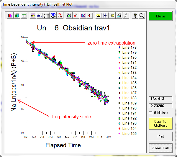
Obviously the totals are low, so we might suspect a TDI situation (even though we used a 10 um beam for all the points). If we examine the TDI data (I almost always just leave this acquisition option turned on because it uses very little overhead, and if you do run into a TDI situation you already have the intensity interval data to perform a TDI correction), you'll see a significant decrease in the Na intensities over time as seen here:

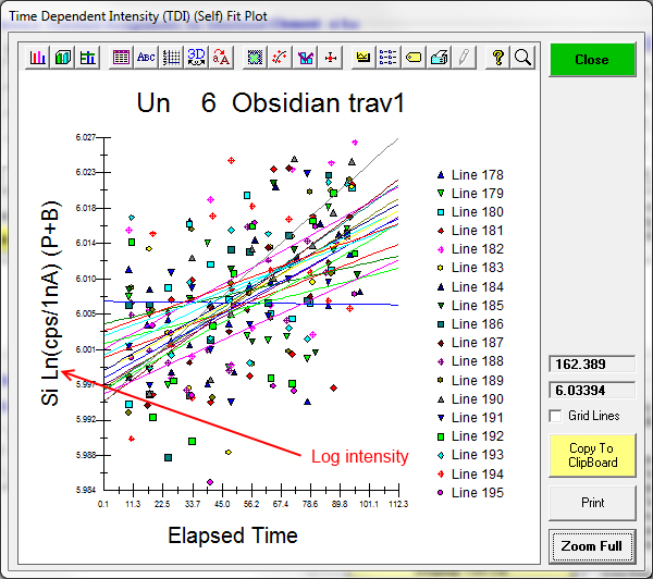
For Si ka the situation is less dire (and is barely statistically significant), but worth a correction:

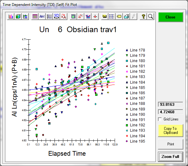
Al ka is somewhat more statistically significant as seen here:

The results for these linear (exponential) extrapolations are seen here:

Un 6 Obsidian trav1, Results in Elemental Weight Percents ELEM: Na Si K Al Mg Fe Ca Sr Mn S Cl Ti P Zr O H TYPE: ANAL ANAL ANAL ANAL ANAL ANAL ANAL ANAL ANAL ANAL ANAL ANAL ANAL ANAL CALC SPEC BGDS: MAN MAN LIN MAN MAN MAN MAN LIN LIN LIN LIN LIN EXP EXP TIME: 90.00 60.00 20.00 80.00 60.00 160.00 80.00 40.00 30.00 100.00 100.00 100.00 100.00 100.00 BEAM: 9.99 9.99 9.99 9.99 9.99 9.99 9.99 9.99 9.99 50.29 50.29 50.29 50.29 50.29 ELEM: Na Si K Al Mg Fe Ca Sr Mn S Cl Ti P Zr O H SUM 178 3.458 35.730 3.773 7.123 .025 .509 .356 .061 .071 .002 .044 .036 .001 -.010 49.379 .000 100.556 179 3.582 35.538 3.941 6.956 .017 .467 .351 .008 .048 .003 .046 .045 -.004 -.011 49.052 .000 100.038 180 3.500 35.492 3.746 6.986 .019 .428 .364 .018 .046 .003 .042 .028 -.004 .006 48.949 .000 99.621 181 3.414 35.456 3.844 6.899 .018 .454 .362 .034 .055 -.001 .039 .050 -.003 -.009 48.843 .000 99.455 182 3.611 35.556 3.657 7.047 .022 .476 .369 -.018 .053 -.001 .041 .027 .000 -.008 49.110 .000 99.943 183 3.451 35.456 3.873 7.107 .023 .487 .371 .000 .058 -.001 .040 .037 -.003 -.006 49.050 .000 99.944 184 3.550 35.447 3.738 6.971 .020 .501 .358 -.003 .064 .002 .035 .038 -.003 .001 48.927 .000 99.646 185 3.516 35.604 3.797 6.893 .024 .414 .365 -.008 .040 .002 .036 .020 -.001 -.020 48.993 .000 99.676 186 3.600 35.384 3.810 7.045 .026 .428 .363 -.014 .039 .001 .033 .037 .000 .000 48.933 .000 99.685 187 3.442 35.291 3.888 6.912 .024 .454 .354 .044 .033 .000 .036 .042 -.005 -.010 48.673 .000 99.178 188 3.502 35.386 3.720 7.048 .017 .406 .351 .033 .040 .001 .034 .023 .000 -.002 48.865 .000 99.424 189 3.609 35.398 3.754 7.058 .020 .376 .355 .010 .029 .001 .033 .030 .003 -.006 48.927 .000 99.596 190 3.459 35.330 3.871 7.052 .018 .453 .343 .036 .042 .002 .033 .027 -.006 -.015 48.824 .000 99.469 191 3.454 35.410 3.676 6.966 .020 .477 .351 .004 .047 -.002 .034 .039 -.002 -.020 48.815 .000 99.269 192 3.526 35.369 3.813 6.985 .020 .488 .360 .040 .063 -.001 .034 .034 -.001 -.006 48.860 .000 99.586 193 3.650 35.608 3.663 7.046 .021 .452 .366 .034 .051 .000 .034 .031 .000 -.012 49.184 .000 100.128 194 3.528 35.638 3.694 7.110 .020 .512 .351 -.011 .055 -.001 .035 .020 -.002 -.008 49.234 .000 100.175 195 3.533 35.369 3.739 7.109 .017 .472 .352 .067 .040 .000 .035 .049 .004 -.018 48.959 .000 99.728 AVER: 3.521 35.470 3.778 7.017 .021 .459 .358 .018 .049 .001 .037 .034 -.001 -.009 48.977 .000 99.729 SDEV: .068 .119 .083 .074 .003 .037 .008 .026 .011 .002 .004 .009 .003 .007 .170 .000 .347 SERR: .016 .028 .020 .017 .001 .009 .002 .006 .003 .000 .001 .002 .001 .002 .040 .000 %RSD: 1.94 .34 2.19 1.06 14.11 8.09 2.12 140.65 23.09 265.87 10.91 26.43 -199.11 -82.49 .35 .00 STDS: 336 14 374 160 162 162 162 251 25 730 285 22 285 257 0 0 STKF: .0735 .4101 .1132 .0334 .0568 .0950 .1027 .4268 .7341 .5061 .0601 .5547 .1599 .4201 .0000 .0000 STCT: 70.51 567.11 225.51 62.06 81.21 18.46 161.20 292.31 2053.05 449.51 79.86 58.15 227.12 213.15 .00 .00 UNKF: .0195 .2914 .0328 .0552 .0001 .0038 .0032 .0001 .0004 .0000 .0003 .0003 .0000 -.0001 .0000 .0000 UNCT: 18.68 403.03 65.30 102.52 .20 .74 5.02 .10 1.12 .00 .39 .03 -.01 -.03 .00 .00 UNBG: .32 .22 .94 .88 .51 .23 1.01 .94 4.78 .16 .33 .05 .81 .88 .00 .00 ZCOR: 1.8086 1.2170 1.1526 1.2706 1.4508 1.1979 1.1182 1.2346 1.2173 1.2854 1.2525 1.1969 1.4626 1.4590 .0000 .0000 KRAW: .2649 .7107 .2896 1.6521 .0025 .0403 .0312 .0004 .0005 .0000 .0049 .0005 -.0001 -.0001 .0000 .0000 PKBG: 59.19 1852.27 70.83 117.93 1.40 4.30 5.98 1.12 1.24 1.03 2.20 1.65 .98 .97 .00 .00 INT%: ---- ---- ---- ---- ---- -.02 ---- -93.93 ---- ---- ---- ---- ---- ---- ---- ---- TDI%: 88.751 -.772 -.008 -1.945 ---- -.173 ---- ---- ---- ---- ---- ---- ---- ---- ---- ---- DEV%: 5.8 .7 2.8 1.2 ---- 8.4 ---- ---- ---- ---- ---- ---- ---- ---- ---- ---- TDIF: LINEAR LINEAR LINEAR LINEAR ---- LINEAR ---- ---- ---- ---- ---- ---- ---- ---- ---- ---- TDIT: 125.56 97.78 61.11 117.28 ---- 198.17 ---- ---- ---- ---- ---- ---- ---- ---- ---- ---- TDII: 18.5 403. 66.2 103. ---- .963 ---- ---- ---- ---- ---- ---- ---- ---- ---- ----

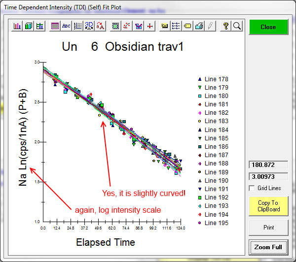
The totals look good, but are we done? Well if we look more closely at the Na TDI plot above, we see that there seems to be a slight curvature in the linear (exponential) fit, so maybe we should utilize the quadratic fit in log space or "hyper-exponential" fit as seen here:

How does this tiny change affect our results? Not that much, but a little. Note the difference in the average deviation in the linear and quadratic fits for Na. The linear (conventional exponential fit) has a DEV% of 5.8, while the "hyper-exponential" (quadratic exponential fit) has a DEV% of 3.4, so the hyper-exponential is definitetely a better fit to the data as seen here:

Un 6 Obsidian trav1, Results in Elemental Weight Percents ELEM: Na Si K Al Mg Fe Ca Sr Mn S Cl Ti P Zr O H TYPE: ANAL ANAL ANAL ANAL ANAL ANAL ANAL ANAL ANAL ANAL ANAL ANAL ANAL ANAL CALC SPEC BGDS: MAN MAN LIN MAN MAN MAN MAN LIN LIN LIN LIN LIN EXP EXP TIME: 90.00 60.00 20.00 80.00 60.00 160.00 80.00 40.00 30.00 100.00 100.00 100.00 100.00 100.00 BEAM: 9.99 9.99 9.99 9.99 9.99 9.99 9.99 9.99 9.99 50.29 50.29 50.29 50.29 50.29 ELEM: Na Si K Al Mg Fe Ca Sr Mn S Cl Ti P Zr O H SUM 178 3.348 35.718 3.773 7.118 .025 .509 .356 .061 .071 .002 .044 .036 .001 -.010 49.322 .000 100.373 179 3.491 35.527 3.941 6.952 .017 .467 .351 .008 .048 .003 .046 .045 -.004 -.011 49.004 .000 99.885 180 3.286 35.467 3.747 6.976 .018 .428 .364 .018 .046 .003 .042 .028 -.004 .006 48.838 .000 99.264 181 3.284 35.442 3.844 6.893 .018 .454 .362 .034 .055 -.001 .039 .050 -.003 -.009 48.776 .000 99.238 182 3.335 35.524 3.658 7.035 .022 .476 .369 -.018 .053 -.001 .041 .027 .000 -.008 48.967 .000 99.481 183 3.360 35.446 3.873 7.103 .023 .487 .371 .000 .058 -.001 .040 .037 -.003 -.006 49.003 .000 99.790 184 3.379 35.427 3.739 6.964 .020 .501 .358 -.003 .064 .002 .035 .038 -.003 .001 48.839 .000 99.361 185 3.540 35.606 3.797 6.895 .024 .414 .365 -.008 .040 .002 .036 .020 -.001 -.020 49.006 .000 99.717 186 3.517 35.375 3.810 7.041 .026 .428 .363 -.014 .039 .001 .033 .037 .000 .000 48.890 .000 99.545 187 3.432 35.290 3.888 6.912 .024 .454 .354 .044 .033 .000 .036 .042 -.005 -.010 48.668 .000 99.161 188 3.320 35.365 3.720 7.040 .017 .406 .351 .033 .040 .001 .034 .023 .000 -.002 48.771 .000 99.118 189 3.309 35.364 3.754 7.044 .020 .376 .355 .010 .029 .001 .033 .030 .003 -.006 48.772 .000 99.094 190 3.479 35.332 3.871 7.053 .018 .453 .343 .036 .042 .002 .033 .027 -.006 -.015 48.834 .000 99.501 191 3.412 35.405 3.676 6.964 .020 .477 .351 .004 .047 -.002 .034 .039 -.002 -.020 48.793 .000 99.198 192 3.431 35.358 3.813 6.981 .019 .488 .360 .040 .063 -.001 .034 .034 -.001 -.006 48.811 .000 99.427 193 3.423 35.582 3.663 7.036 .020 .452 .366 .034 .051 .000 .034 .031 .000 -.012 49.066 .000 99.747 194 3.390 35.623 3.695 7.104 .020 .512 .351 -.011 .055 -.001 .035 .020 -.002 -.008 49.163 .000 99.944 195 3.324 35.346 3.740 7.099 .017 .472 .352 .067 .040 .000 .035 .049 .004 -.018 48.851 .000 99.379 AVER: 3.392 35.455 3.778 7.012 .020 .459 .358 .019 .049 .001 .037 .034 -.001 -.009 48.910 .000 99.512 SDEV: .079 .118 .083 .073 .003 .037 .008 .026 .011 .002 .004 .009 .003 .007 .162 .000 .341 SERR: .019 .028 .019 .017 .001 .009 .002 .006 .003 .000 .001 .002 .001 .002 .038 .000 %RSD: 2.32 .33 2.19 1.03 14.25 8.09 2.12 140.57 23.09 265.88 10.91 26.43 -199.12 -82.46 .33 .00 STDS: 336 14 374 160 162 162 162 251 25 730 285 22 285 257 0 0 STKF: .0735 .4101 .1132 .0334 .0568 .0950 .1027 .4268 .7341 .5061 .0601 .5547 .1599 .4201 .0000 .0000 STCT: 70.51 567.11 225.51 62.06 81.21 18.46 161.20 292.31 2053.05 449.51 79.86 58.15 227.12 213.15 .00 .00 UNKF: .0187 .2914 .0328 .0552 .0001 .0038 .0032 .0001 .0004 .0000 .0003 .0003 .0000 -.0001 .0000 .0000 UNCT: 17.98 403.03 65.30 102.52 .20 .74 5.02 .10 1.12 .00 .39 .03 -.01 -.03 .00 .00 UNBG: .32 .22 .94 .88 .51 .23 1.01 .94 4.78 .16 .33 .05 .81 .88 .00 .00 ZCOR: 1.8095 1.2165 1.1527 1.2696 1.4493 1.1979 1.1183 1.2342 1.2174 1.2855 1.2526 1.1969 1.4627 1.4597 .0000 .0000 KRAW: .2550 .7107 .2896 1.6521 .0025 .0403 .0312 .0004 .0005 .0000 .0049 .0005 -.0001 -.0001 .0000 .0000 PKBG: 57.04 1851.22 70.83 117.83 1.39 4.30 5.97 1.12 1.24 1.03 2.20 1.65 .98 .97 .00 .00 INT%: ---- ---- ---- ---- ---- -.02 ---- -93.93 ---- ---- ---- ---- ---- ---- ---- ---- TDI%: 81.846 -.772 -.008 -1.945 ---- -.173 ---- ---- ---- ---- ---- ---- ---- ---- ---- ---- DEV%: 3.4 .7 2.8 1.2 ---- 8.4 ---- ---- ---- ---- ---- ---- ---- ---- ---- ---- TDIF: QUADRA LINEAR LINEAR LINEAR ---- LINEAR ---- ---- ---- ---- ---- ---- ---- ---- ---- ---- TDIT: 125.56 97.78 61.11 117.28 ---- 198.17 ---- ---- ---- ---- ---- ---- ---- ---- ---- ---- TDII: 18.3 403. 66.2 103. ---- .963 ---- ---- ---- ---- ---- ---- ---- ---- ---- ----

And our Na value went from 3.5 wt% to just under 3.4 wt%. Not much, remember the fit is better, so it should be a better extrapolation.

Now what about Ed's point about the early TDI intervals being more important for the extrapolation?

If we pull up the Analytical | Analysis Options menu dialog, in addition to a global flag for toggling all TDI corrections in the run, we also see the Use Time Weighted data for TFI Fit option. Let's turn that on and use the default 8 weighting factor which means that the first TDI point will be duplicated 8 times, the 2nd TDI point 7 times, the 3rd TDI point 6 times, etc., etc., before being fit!

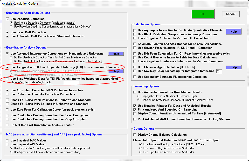
Now what does our Na data look like?

Un 6 Obsidian trav1, Results in Elemental Weight Percents ELEM: Na Si K Al Mg Fe Ca Sr Mn S Cl Ti P Zr O H TYPE: ANAL ANAL ANAL ANAL ANAL ANAL ANAL ANAL ANAL ANAL ANAL ANAL ANAL ANAL CALC SPEC BGDS: MAN MAN LIN MAN MAN MAN MAN LIN LIN LIN LIN LIN EXP EXP TIME: 90.00 60.00 20.00 80.00 60.00 160.00 80.00 40.00 30.00 100.00 100.00 100.00 100.00 100.00 BEAM: 9.99 9.99 9.99 9.99 9.99 9.99 9.99 9.99 9.99 50.29 50.29 50.29 50.29 50.29 ELEM: Na Si K Al Mg Fe Ca Sr Mn S Cl Ti P Zr O H SUM 178 3.086 35.654 3.801 7.090 .025 .497 .356 .061 .071 .002 .044 .036 .001 -.010 49.135 .000 99.848 179 3.321 35.488 3.953 6.886 .017 .483 .351 .008 .048 .003 .046 .045 -.004 -.011 48.849 .000 99.483 180 3.273 35.258 3.674 7.076 .018 .417 .364 .020 .046 .003 .042 .028 -.004 .006 48.666 .000 98.887 181 3.121 35.403 3.897 6.847 .018 .480 .362 .034 .055 -.001 .039 .050 -.003 -.009 48.652 .000 98.946 182 3.300 35.628 3.621 6.982 .022 .534 .369 -.019 .053 -.001 .041 .027 .000 -.008 49.035 .000 99.584 183 3.354 35.546 3.822 7.081 .023 .494 .371 -.001 .058 -.001 .040 .037 -.003 -.006 49.088 .000 99.904 184 3.277 35.309 3.695 6.935 .020 .471 .358 -.003 .064 .002 .035 .038 -.003 .001 48.626 .000 98.824 185 3.450 35.538 3.764 6.835 .024 .418 .365 -.008 .040 .002 .036 .020 -.001 -.020 48.838 .000 99.302 186 3.465 35.431 3.717 7.048 .026 .441 .363 -.015 .039 .001 .033 .037 .000 .000 48.925 .000 99.510 187 3.366 35.184 3.895 6.827 .024 .475 .354 .044 .033 .000 .036 .042 -.005 -.010 48.456 .000 98.721 188 3.155 35.356 3.740 6.979 .016 .392 .351 .033 .040 .001 .034 .023 .000 -.002 48.649 .000 98.768 189 3.186 35.214 3.775 7.030 .020 .372 .355 .011 .029 .001 .033 .030 .003 -.006 48.549 .000 98.601 190 3.365 35.294 3.854 7.085 .017 .473 .343 .036 .042 .002 .033 .027 -.006 -.015 48.783 .000 99.335 191 3.305 35.340 3.648 6.952 .020 .475 .351 .004 .047 -.002 .034 .039 -.002 -.020 48.664 .000 98.854 192 3.403 35.474 3.750 6.899 .019 .460 .360 .039 .063 -.001 .034 .034 -.001 -.006 48.840 .000 99.371 193 3.304 35.654 3.683 7.005 .020 .446 .366 .033 .051 .000 .034 .031 .000 -.012 49.082 .000 99.699 194 3.209 35.320 3.662 7.111 .020 .539 .351 -.009 .055 -.001 .035 .020 -.002 -.008 48.762 .000 99.064 195 3.181 35.328 3.741 7.089 .017 .476 .352 .067 .040 .000 .035 .049 .004 -.018 48.774 .000 99.136 AVER: 3.284 35.412 3.761 6.987 .020 .464 .358 .019 .049 .001 .037 .034 -.001 -.009 48.798 .000 99.213 SDEV: .110 .148 .094 .097 .003 .044 .008 .026 .011 .002 .004 .009 .003 .007 .195 .000 .403 SERR: .026 .035 .022 .023 .001 .010 .002 .006 .003 .000 .001 .002 .001 .002 .046 .000 %RSD: 3.33 .42 2.50 1.38 14.35 9.44 2.12 138.43 23.09 265.87 10.91 26.43 -199.12 -82.49 .40 .00 STDS: 336 14 374 160 162 162 162 251 25 730 285 22 285 257 0 0 STKF: .0735 .4101 .1132 .0334 .0568 .0950 .1027 .4268 .7341 .5061 .0601 .5547 .1599 .4201 .0000 .0000 STCT: 71.55 568.51 226.21 62.09 81.21 18.33 161.20 292.31 2053.05 449.51 79.86 58.15 227.12 213.15 .00 .00 UNKF: .0181 .2912 .0326 .0551 .0001 .0039 .0032 .0002 .0004 .0000 .0003 .0003 .0000 -.0001 .0000 .0000 UNCT: 17.66 403.69 65.20 102.27 .20 .75 5.02 .10 1.12 .00 .39 .03 -.01 -.03 .00 .00 UNBG: .32 .22 .94 .88 .51 .23 1.01 .94 4.78 .16 .33 .05 .81 .88 .00 .00 ZCOR: 1.8103 1.2161 1.1528 1.2688 1.4481 1.1980 1.1184 1.2337 1.2174 1.2857 1.2528 1.1970 1.4629 1.4594 .0000 .0000 KRAW: .2468 .7101 .2882 1.6472 .0025 .0407 .0312 .0004 .0005 .0000 .0049 .0005 -.0001 -.0001 .0000 .0000 PKBG: 56.05 1853.28 70.71 117.47 1.39 4.31 5.97 1.12 1.24 1.03 2.20 1.65 .98 .97 .00 .00 INT%: ---- ---- ---- ---- ---- -.02 ---- -93.84 ---- ---- ---- ---- ---- ---- ---- ---- TDI%: 78.615 -.609 -.162 -2.187 ---- .092 ---- ---- ---- ---- ---- ---- ---- ---- ---- ---- DEV%: 2.5 .7 2.5 1.2 ---- 7.6 ---- ---- ---- ---- ---- ---- ---- ---- ---- ---- TDIF: QUADRA LINEAR LINEAR LINEAR ---- LINEAR ---- ---- ---- ---- ---- ---- ---- ---- ---- ---- TDIT: 125.56 97.78 61.11 117.28 ---- 198.17 ---- ---- ---- ---- ---- ---- ---- ---- ---- ---- TDII: 18.0 404. 66.1 103. ---- .965 ---- ---- ---- ---- ---- ---- ---- ---- ---- ----

I have to say I was surprised. The time weighted data option had more effect on the data that the hyper-exponential fit (on this dataset anyway), because Na went from 3.4 wt% to 3.28 wt% *and* the overall DEV% improved to 2.5.

So, yes, Ed is correct, we should give our first TDI intervals more "weight" one way or another.

Probeman · « **Reply #8 on:** November 28, 2013, 11:31:56 AM »

And now for something completely different!

A student recently analyzed a fiber optic as a class project and it was interesting to see the TDI effects for pure SiO2 crystal versus glass. For example, if we use SiO2 as a standard and acquire the standard also as an unknown, we get reasonable results because the TDI effects on the Si Ka and O ka are almost normalized out as seen here:

Un 7 SiO2 synthetic TakeOff = 40.0 KiloVolt = 15.0 Beam Current = 50.0 Beam Size = 10 (Magnification (analytical) = 40000), Beam Mode = Analog Spot (Magnification (default) = 400, Magnification (imaging) = 800) Image Shift (X,Y): .00, .00 Number of Data Lines: 5 Number of 'Good' Data Lines: 5 First/Last Date-Time: 11/27/2013 04:57:01 PM to 11/27/2013 05:21:02 PM WARNING- Using Exponential Off-Peak correction for si ka WARNING- Using Exponential Off-Peak correction for o ka Average Total Oxygen: .000 Average Total Weight%: 99.708 Average Calculated Oxygen: .000 Average Atomic Number: 10.798 Average Excess Oxygen: .000 Average Atomic Weight: 20.020 Oxygen Equiv. from Halogen: .000 Halogen Corrected Oxygen: .000 Average ZAF Iteration: 7.00 Average Quant Iterate: 2.00 Un 7 SiO2 synthetic, Results in Elemental Weight Percents ELEM: Si O Er Cl BGDS: EXP EXP LIN LIN TIME: 40.00 40.00 160.00 160.00 BEAM: 50.09 50.09 50.09 50.09 ELEM: Si O Er Cl SUM 169 46.586 53.121 -.001 -.001 99.705 170 46.491 53.288 -.002 .001 99.777 171 46.521 53.079 .008 .000 99.607 172 46.599 53.152 -.009 .002 99.745 173 46.459 53.260 -.013 .000 99.706 AVER: 46.531 53.180 -.003 .000 99.708 SDEV: .060 .090 .008 .001 .064 SERR: .027 .040 .004 .001 %RSD: .13 .17 -235.67 745.15 STDS: 14 14 1003 285 STKF: .4101 .2664 .5350 .0601 STCT: 693.09 267.64 184.31 43.90 UNKF: .4082 .2661 .0000 .0000 UNCT: 689.96 267.40 -.01 .00 UNBG: 1.00 1.44 .82 .22 ZCOR: 1.1398 1.9985 1.5611 1.2798 KRAW: .9955 .9991 .0000 .0000 PKBG: 692.47 186.37 .99 1.01

In addition to the TDI effects being similar (because we are analyzing the same material for both standard and unknown), they are also fairly minor in magnitude as seen here for Si Ka in SiO2 crystal:

One could even argue we are "over fitting" the Si Ka TDI correction because it is such a small correction. Which is *not* the case for O Ka in SiO2 crystal:

As has been observed by many, the oxygen intensity changes dramatically over time even with a 10 um diameter beam. In fact the TDI effect for O Ka is very dependent on subtle surface conditions such as the carbon coat. Because of this, with the TDI correction turned on for both the standard SiO2 and the same standard acquired as an unknown, we get these somewhat improved results for SiO2 analyzed as an unknown:

Un 7 SiO2 synthetic TakeOff = 40.0 KiloVolt = 15.0 Beam Current = 50.0 Beam Size = 10 (Magnification (analytical) = 40000), Beam Mode = Analog Spot (Magnification (default) = 400, Magnification (imaging) = 800) Image Shift (X,Y): .00, .00 Number of Data Lines: 5 Number of 'Good' Data Lines: 5 First/Last Date-Time: 11/27/2013 04:57:01 PM to 11/27/2013 05:21:02 PM WARNING- Using Exponential Off-Peak correction for si ka WARNING- Using Exponential Off-Peak correction for o ka WARNING- Using Time Dependent Intensity (TDI) Element Correction Average Total Oxygen: .000 Average Total Weight%: 99.846 Average Calculated Oxygen: .000 Average Atomic Number: 10.800 Average Excess Oxygen: .000 Average Atomic Weight: 20.024 Oxygen Equiv. from Halogen: .000 Halogen Corrected Oxygen: .000 Average ZAF Iteration: 7.00 Average Quant Iterate: 2.00 Un 7 SiO2 synthetic, Results in Elemental Weight Percents ELEM: Si O Er Cl BGDS: EXP EXP LIN LIN TIME: 40.00 40.00 160.00 160.00 BEAM: 50.09 50.09 50.09 50.09 ELEM: Si O Er Cl SUM 169 46.629 53.392 -.001 -.001 100.019 170 46.641 53.254 -.002 .001 99.893 171 46.414 53.376 .007 .000 99.797 172 46.619 52.784 -.009 .002 99.397 173 46.856 53.279 -.013 .000 100.122 AVER: 46.632 53.217 -.003 .000 99.846 SDEV: .157 .249 .008 .001 .280 SERR: .070 .111 .004 .001 %RSD: .34 .47 -230.82 747.92 STDS: 14 14 1003 285 STKF: .4101 .2664 .5350 .0601 STCT: 699.38 249.93 184.41 50.55 UNKF: .4092 .2662 .0000 .0000 UNCT: 697.79 249.77 -.01 .00 UNBG: 1.00 1.44 .82 .22 ZCOR: 1.1397 1.9993 1.5466 1.2799 KRAW: .9977 .9993 .0000 .0000 PKBG: 700.33 174.14 .99 1.01 TDI%: 1.135 -6.591 -.632 -.248 DEV%: .1 .2 .2 1.3 TDIF: QUADRA QUADRA LINEAR LINEAR TDIT: 51.40 51.80 170.20 170.20 TDII: 698. 250. .823 .220

From this we might conclude that even when analyzing the *same* material, it is sometimes necessary to run *both* the standard and unknown not only at similar beam conditions, but also utilizing the TDI acquisition and correction for both standard and unknown because of subtle variations in coating, adsorbed water, beam focus and thermal conductivity (etc.?).

Probeman · « **Reply #9 on:** December 05, 2013, 12:43:39 PM »

Ok, so I was able to do a quick run of SiO2 crystal versus SiO2 glass and here are the results. Conditions (using the Analyze! "Report" button) were:

Compositional analyses were acquired on an electron microprobe (Cameca SX100 (TCP/IP Socket)) equipped with 5 tunable wavelength dispersive spectrometers. Operating conditions were 40 degrees takeoff angle, and a beam energy of 15 keV. The beam current was 50 nA, and the beam diameter was 10 microns.

Elements were acquired using analyzing crystals LPET for Cl ka, LTAP for Al ka, TAP for Si ka, and PC1 for O ka.

The standards were Ca10(PO4)6Cl2 (halogen corrected) for Cl ka, Nepheline (partial anal.) for Al ka, and SiO2 (elemental) (#14) for Si ka, O ka.

The counting time was 60 seconds for all elements. The intensity data was corrected for Time Dependent Intensity (TDI) loss (or gain) using a self calibrated correction for Si ka, O ka, Al ka, Cl ka. The off peak counting time was 20 seconds for all elements. Off Peak correction method was Linear for Cl ka, and Exponential for O ka, Al ka, Si ka.

Unknown and standard intensities were corrected for deadtime. Standard intensities were corrected for standard drift over time.

The exponential or polynomial background fit was utilized. See John J. Donovan, Heather A. Lowers and Brian G. Rusk, Improved electron probe microanalysis of trace elements in quartz, American Mineralogist, 96, 2011

The SiO2 crystal acquisition for Si Ka looks like this:

The SiO2 crystal acquisition for O Ka looks like this:

The SiO2 glass acquisition for Si Ka looks like this:

The SiO2 glass acquisition for O Ka looks like this:

The quant results running both materials as unknowns (using SiO2 crystal as the primary standard) is here w/o the TDI correction:

Un 2 SiO2 xtal TakeOff = 40.0 KiloVolt = 15.0 Beam Current = 50.0 Beam Size = 10 (Magnification (analytical) = 40000), Beam Mode = Analog Spot (Magnification (default) = 400, Magnification (imaging) = 800) Image Shift (X,Y): .00, .00 Number of Data Lines: 5 Number of 'Good' Data Lines: 5 First/Last Date-Time: 12/03/2013 02:48:14 PM to 12/03/2013 02:57:40 PM WARNING- Using Exponential Off-Peak correction for si ka WARNING- Using Exponential Off-Peak correction for o ka WARNING- Using Exponential Off-Peak correction for al ka Average Total Oxygen: .000 Average Total Weight%: 100.309 Average Calculated Oxygen: .000 Average Atomic Number: 10.799 Average Excess Oxygen: .000 Average Atomic Weight: 20.019 Oxygen Equiv. from Halogen: .000 Halogen Corrected Oxygen: .000 Average ZAF Iteration: 7.00 Average Quant Iterate: 2.00 Un 2 SiO2 xtal, Results in Elemental Weight Percents ELEM: Si O Al Cl BGDS: EXP EXP EXP LIN TIME: 60.00 60.00 60.00 60.00 BEAM: 49.82 49.82 49.82 49.82 ELEM: Si O Al Cl SUM 117 46.791 53.450 .005 .001 100.247 118 46.767 53.493 .000 .000 100.259 119 46.849 53.574 .001 .000 100.425 120 46.774 53.489 .000 .003 100.266 121 46.785 53.559 .005 .001 100.350 AVER: 46.793 53.513 .002 .001 100.309 SDEV: .033 .052 .003 .001 .076 SERR: .015 .023 .001 .001 %RSD: .07 .10 121.62 104.43 STDS: 914 914 336 285 STKF: .4101 .2664 .1331 .0601 STCT: 687.69 250.10 724.87 78.57 UNKF: .4105 .2678 .0000 .0000 UNCT: 688.37 251.44 .10 .01 UNBG: .98 1.38 3.19 .32 ZCOR: 1.1399 1.9982 1.2289 1.2798 KRAW: 1.0010 1.0053 .0001 .0002 PKBG: 704.90 183.81 1.03 1.04 Un 3 SiO2 glass TakeOff = 40.0 KiloVolt = 15.0 Beam Current = 50.0 Beam Size = 10 (Magnification (analytical) = 40000), Beam Mode = Analog Spot (Magnification (default) = 400, Magnification (imaging) = 800) Image Shift (X,Y): .00, .00 Number of Data Lines: 5 Number of 'Good' Data Lines: 5 First/Last Date-Time: 12/03/2013 03:00:25 PM to 12/03/2013 03:09:47 PM WARNING- Using Exponential Off-Peak correction for si ka WARNING- Using Exponential Off-Peak correction for o ka WARNING- Using Exponential Off-Peak correction for al ka Average Total Oxygen: .000 Average Total Weight%: 99.375 Average Calculated Oxygen: .000 Average Atomic Number: 10.811 Average Excess Oxygen: .000 Average Atomic Weight: 20.040 Average ZAF Iteration: 7.00 Average Quant Iterate: 2.00 Un 3 SiO2 glass, Results in Elemental Weight Percents ELEM: Si O Al Cl BGDS: EXP EXP EXP LIN TIME: 60.00 60.00 60.00 60.00 BEAM: 49.82 49.82 49.82 49.82 ELEM: Si O Al Cl SUM 122 46.514 52.881 .004 .004 99.403 123 46.538 52.747 .004 -.003 99.285 124 46.572 52.861 .006 -.003 99.436 125 46.540 52.787 .005 -.003 99.329 126 46.586 52.829 .006 .002 99.423 AVER: 46.550 52.821 .005 .000 99.375 SDEV: .029 .055 .001 .003 .065 SERR: .013 .024 .000 .001 %RSD: .06 .10 23.08 -815.86 STDS: 914 914 336 285 STKF: .4101 .2664 .1331 .0601 STCT: 687.97 250.02 725.07 78.20 UNKF: .4086 .2637 .0000 .0000 UNCT: 685.39 247.54 .21 .00 UNBG: .97 1.28 3.17 .32 ZCOR: 1.1394 2.0028 1.2278 1.2803 KRAW: .9962 .9901 .0003 -.0001 PKBG: 705.66 194.79 1.07 1.00

The SiO2 crystal looks fine because it was run at the exact same conditions as the SiO2 (crystal) standard, but the SiO2 glass is a little low in oxygen due to the different TDI effects for glass.

The quant results running both materials as unknowns (using SiO2 crystal as the primary standard) is here with the TDI correction:

Un 2 SiO2 xtal TakeOff = 40.0 KiloVolt = 15.0 Beam Current = 50.0 Beam Size = 10 (Magnification (analytical) = 40000), Beam Mode = Analog Spot (Magnification (default) = 400, Magnification (imaging) = 800) Image Shift (X,Y): .00, .00 Number of Data Lines: 5 Number of 'Good' Data Lines: 5 First/Last Date-Time: 12/03/2013 02:48:14 PM to 12/03/2013 02:57:40 PM WARNING- Using Exponential Off-Peak correction for si ka WARNING- Using Exponential Off-Peak correction for o ka WARNING- Using Exponential Off-Peak correction for al ka WARNING- Using Time Dependent Intensity (TDI) Element Correction Average Total Oxygen: .000 Average Total Weight%: 100.335 Average Calculated Oxygen: .000 Average Atomic Number: 10.802 Average Excess Oxygen: .000 Average Atomic Weight: 20.024 Oxygen Equiv. from Halogen: .000 Halogen Corrected Oxygen: .000 Average ZAF Iteration: 7.00 Average Quant Iterate: 2.00 Un 2 SiO2 xtal, Results in Elemental Weight Percents ELEM: Si O Al Cl BGDS: EXP EXP EXP LIN TIME: 60.00 60.00 60.00 60.00 BEAM: 49.82 49.82 49.82 49.82 ELEM: Si O Al Cl SUM 117 46.871 53.523 .005 .001 100.400 118 46.788 53.315 .000 .000 100.102 119 46.907 53.558 .001 .000 100.466 120 46.786 53.323 .000 .003 100.113 121 46.931 53.658 .005 .001 100.595 AVER: 46.857 53.475 .002 .001 100.335 SDEV: .067 .151 .003 .001 .219 SERR: .030 .068 .001 .001 %RSD: .14 .28 121.49 112.65 STDS: 914 914 336 285 STKF: .4101 .2664 .1331 .0601 STCT: 689.39 243.24 724.48 83.43 UNKF: .4111 .2675 .0000 .0000 UNCT: 691.10 244.22 .10 .01 UNBG: .98 1.38 3.19 .32 ZCOR: 1.1397 1.9994 1.2286 1.2799 KRAW: 1.0025 1.0040 .0001 .0001 PKBG: 707.67 178.58 1.03 1.04 TDI%: .396 -2.869 -.408 -.238 DEV%: .3 .4 2.5 9.2 TDIF: LINEAR QUADRA LINEAR LINEAR TDIT: 84.20 84.60 83.60 84.20 TDII: 692. 244. 3.27 .331 Un 3 SiO2 glass TakeOff = 40.0 KiloVolt = 15.0 Beam Current = 50.0 Beam Size = 10 (Magnification (analytical) = 40000), Beam Mode = Analog Spot (Magnification (default) = 400, Magnification (imaging) = 800) Image Shift (X,Y): .00, .00 Number of Data Lines: 5 Number of 'Good' Data Lines: 5 First/Last Date-Time: 12/03/2013 03:00:25 PM to 12/03/2013 03:09:47 PM WARNING- Using Exponential Off-Peak correction for si ka WARNING- Using Exponential Off-Peak correction for o ka WARNING- Using Exponential Off-Peak correction for al ka WARNING- Using Time Dependent Intensity (TDI) Element Correction Average Total Oxygen: .000 Average Total Weight%: 100.645 Average Calculated Oxygen: .000 Average Atomic Number: 10.773 Average Excess Oxygen: .000 Average Atomic Weight: 19.971 Average ZAF Iteration: 7.00 Average Quant Iterate: 2.00 Un 3 SiO2 glass, Results in Elemental Weight Percents ELEM: Si O Al Cl BGDS: EXP EXP EXP LIN TIME: 60.00 60.00 60.00 60.00 BEAM: 49.82 49.82 49.82 49.82 ELEM: Si O Al Cl SUM 122 46.507 54.165 .004 .004 100.681 123 46.353 54.176 .004 -.003 100.530 124 46.612 54.116 .006 -.002 100.731 125 46.438 54.070 .005 -.002 100.510 126 46.611 54.154 .006 .002 100.773 AVER: 46.504 54.136 .005 .000 100.645 SDEV: .112 .043 .001 .003 .119 SERR: .050 .019 .001 .001 %RSD: .24 .08 22.98 -944.62 STDS: 914 914 336 285 STKF: .4101 .2664 .1331 .0601 STCT: 689.83 243.44 724.69 83.31 UNKF: .4075 .2724 .0000 .0000 UNCT: 685.50 248.91 .22 .00 UNBG: .97 1.28 3.17 .32 ZCOR: 1.1411 1.9876 1.2313 1.2786 KRAW: .9937 1.0225 .0003 .0000 PKBG: 705.77 195.85 1.07 1.00 TDI%: .016 .554 .656 2.221 DEV%: .3 .4 2.9 3.8 TDIF: LINEAR LINEAR LINEAR LINEAR TDIT: 83.20 84.00 83.20 83.40 TDII: 686. 250. 3.41 .323

Mike Jercinovic · « **Reply #10 on:** February 18, 2014, 06:57:30 AM »

One thing here is that it would be nice to have the button (in std assignments) that now says "remove TDI correction" to default to "add TDI correction", so that it would be done for all TDI-specified elements, sor even better, to invoke the TDI correction by default if it has been checked to use it in Special Options (then you can default the button in std assignments to "remove TDI", but if you do click it, then the button should change to "use TDI".

Right now we still have to click on each element and specify the use of TDI even though we have said to acquire using TDI in Special Options in Acquire. Every time we run an analysis, we have to do this, even though the stored setup had TDI invoked. If we do point by point acquisition and do the TDI specification on the first point of the file, it will turn it off again on the next point, so if we want to look at the numbers as we go, we have to redo the TDI on this file (in std. assignments) after each point.

John Donovan · « **Reply #11 on:** February 18, 2014, 11:59:37 AM »

Quote from: Mike Jercinovic on February 18, 2014, 06:57:30 AM

One thing here is that it would be nice to have the button (in std assignments) that now says "remove TDI correction" to default to "add TDI correction", so that it would be done for all TDI-specified elements, sor even better, to invoke the TDI correction by default if it has been checked to use it in Special Options (then you can default the button in std assignments to "remove TDI", but if you do click it, then the button should change to "use TDI".

Hi Mike,
Let me make sure I understand what you are asking here...

Are you merely saying you want to be able to "toggle" the TDI correction on and off so one can see the analysis with and without TDI correction? If so, you can do that from the Analytical | Analysis Options menu dialog as seen here:

In fact, every correction Probe for EPMA performs on your data can be "toggled" on and off globally for the entire run from this dialog above.

The Remove TDI Correction button in the Standard Assignments dialog actually removes the TDI assignments from the specified samples, so reversing that is problematic (maybe not so much for the *self* TDI correction, but for the *assigned* TDI correction certainly).

Quote from: Mike Jercinovic

Right now we still have to click on each element and specify the use of TDI even though we have said to acquire using TDI in Special Options in Acquire. Every time we run an analysis, we have to do this, even though the stored setup had TDI invoked. If we do point by point acquisition and do the TDI specification on the first point of the file, it will turn it off again on the next point, so if we want to look at the numbers as we go, we have to redo the TDI on this file (in std. assignments) after each point.

If you want to have the TDI assignments used throughout the run simply turn them on in the first sample (even if there's no data) and all subsequent samples should automatically utilize those assignments.

On the other hand, if you're using sample setups to create new samples, make sure the specified sample setup has the TDI assignments are turned on and they should be brought forward.

The program is designed to automatically turn on the TDI assignments automatically when the sample is acquired as seen here:

Of course one can also select all samples and turn on the TDI assignments that way also. I'm probably missing something, so please let me know if I have...

Mike Jercinovic · « **Reply #12 on:** February 18, 2014, 03:10:11 PM »

Well, we are not so much interested in toggling TDI off and on...we just would like TDI to be defaulted to actively being used once we have specified for it to do so. Maybe it's just our system, but once we have a unknown sample setup, and have specified to use TDI in special options, and specified to use TDI in analysis options (quantitative analysis options), then go and click on the standard assignments (in analyze), click on each element we want to use TDI (U, Th, and Pb) and click the button to "use TDI self calibration correction", click OK, then store this unknown sample as a setup (add to setup), then digitize something and specify to use that setup, TDI is NOT used. It acquires as a TDI acquisition, but does not calculate the result using TDI until I go back into standard assignments and tell it to use TDI for those elements again. I just did this with a monazite setup, activating TDI for these elements, then storing that as a setup, then digitizing an analysis using that setup. When I look at the newly acquired data in analyze, going into standard assignments and clicking on U, then Th, then Pb, all of them now have the buttons selected to NOT use TDI. So, we dutifully click each one and re-calculate. There is nothing we seem to be able to do to get it to do this properly, so every time we acquire a new unknown sample, we have to activate TDI use for each of these elements.

John Donovan · « **Reply #13 on:** February 18, 2014, 03:38:17 PM »

Hi Mike,
OK, this is interesting. When I tried it from the Acquire! window this morning with a new run and a new sample it acquired the TDI data and when I went in to look at the intensities, the TDI assignment was already specified as I showed above. Maybe you're not "holding your tongue just right"?

Seriously, let's get to the bottom of this. Try a new test run and new sample from scratch and see if you can reproduce the problem there.

Note: There is a "feature" that uses the existing TDI assignments for new samples (e.g., some turned off/some turned on), so maybe what you're seeing is based on that feature's behavior?

By the way if you select multiple samples, the default assignments that you see in the dialog are based on the *last* sample selected in the Analyze! sample list.

Edit: are the TDI assignments already made to the sample setup used for the acquisition?

Mike Jercinovic · « **Reply #14 on:** February 23, 2014, 08:31:43 AM »

It's probably just us. Here is the first example...
1) start new database
2) new unknown sample (in Acquire), call it monazite setup
3) select new sample from file, navigate to the last database where monazite was run, and pick up an unknown that used, and specified TDI
4) in Acquire, go to special options and make sure that the use TDI button is activated
5) go to analysis options and make sure the use TDI option is checked
6) go to Analyze and then into standard assignments, check whether TDI is activated for U, Th, Pb...it is not, so we activate TDI for each of these elements, click OK with each, then click OK for the main standard assignments window.
7) with this new unknown still highlighted, click to store it as a setup (in Analyze)

go to the Automate window and digitize a new unknown
9) digitize a 6-pt grid
10) specify for this unknown to use the just-stored setup (monazite setup)
11) run the newly digitized sample, making sure that the use specified setups button is active
12) the analysis completes, click OK
13) now go to standard assignments for the newly acquired unknown,
14) for U, Th, and Pb, it shows now that DO NOT USE TDI is active, so we have to then activate TDI (self cal) for each of these elements.

Just to be sure it did not actually do the calculated intensities with TDI even though the TDI buttons are not apparently active, you can run analyze before going back to check the standard assignments to see the results, then go into standard assignments and check the use TDI (self) buttons and re-run analyze. Sure enough, the results change as they should (in this case to very slightly lower the intensities, as counts for these three elements are all slightly increasing with time).

I we now store this new unknown as a setup and use it for digitized samples, the manifestation is the same, TDI will not be active for U, Th, and Pb until we go back into standard assignments and re-specify TDI again.

News:

Author Topic: Improving Time Dependent Intensity (TDI) Corrections (Read 13283 times)

Probeman

Improving Time Dependent Intensity (TDI) Corrections

Probeman

Re: Improving Time Dependent Intensity (TDI) Corrections

Probeman

Re: Improving Time Dependent Intensity (TDI) Corrections

qEd

Re: Improving Time Dependent Intensity (TDI) Corrections

qEd

Re: Improving Time Dependent Intensity (TDI) Corrections

Probeman

Re: Improving Time Dependent Intensity (TDI) Corrections

qEd

Re: Improving Time Dependent Intensity (TDI) Corrections

Probeman

Re: Improving Time Dependent Intensity (TDI) Corrections

Probeman

Re: Improving Time Dependent Intensity (TDI) Corrections

Probeman

Re: Improving Time Dependent Intensity (TDI) Corrections

Mike Jercinovic

Re: Improving Time Dependent Intensity (TDI) Corrections

John Donovan

Re: Improving Time Dependent Intensity (TDI) Corrections

Mike Jercinovic

Re: Improving Time Dependent Intensity (TDI) Corrections

John Donovan

Re: Improving Time Dependent Intensity (TDI) Corrections

Mike Jercinovic

Re: Improving Time Dependent Intensity (TDI) Corrections