I introduced CPQ mapping as a new feature a while back but now think it would be useful to run through the steps to quantify a map using this quant mapping technique. So what exactly is Correlated Pixel Quantification? Basically instead of acquiring a set of discrete data points for our standard intensities we will be acquiring standard intensities in *exactly* the same manner as our unknown x-ray maps. In this way we will construct our k-ratio from the correlation of Ipixel_unkn(i,j) from our unknown map with Ipixel_std(i,j) from our standard x-ray map.
As we all know, generally we will acquire x-ray maps of our areas of interest and point analyses of standard for quantification. But what if there are intrinsic artifacts in the acquisition of our unknown x-ray maps that are not adequately also captured by our point standard intensities? Then the k-ratio produced from Iunk/Istd will not be accurate. How can this occur?
I am currently only aware of two applications for this method, but I'm sure there are many more than have been overlooked, so if any of our members can think of other applications for CPQ mapping I would be most interested to hear any other ideas.
The first application for CPQ is accounting for the carbon contamination dynamic from a high resolution scan for carbon K-alpha (Pinard and Richter). Most instruments, even so called "dry" systems will experience some rate of carbon deposition around the beam impact area. If the standard intensities are not acquired under the same conditions as the unknowns there will be various biases introduced into the k-ratio.
The second application is correcting for WDS Bragg defocusing effects at low beam scan magnifications. This is what we will examine is this post.
First we acquire a set of low mag beam scans on pyrite (FeS2) for Fe Ka and S Ka, as seen here in these plots of the net intensities (remember the continuum is generally fairly flat and so does not experience Bragg defocusing to the same degree as the characteristic peak).
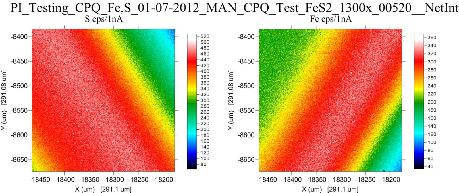
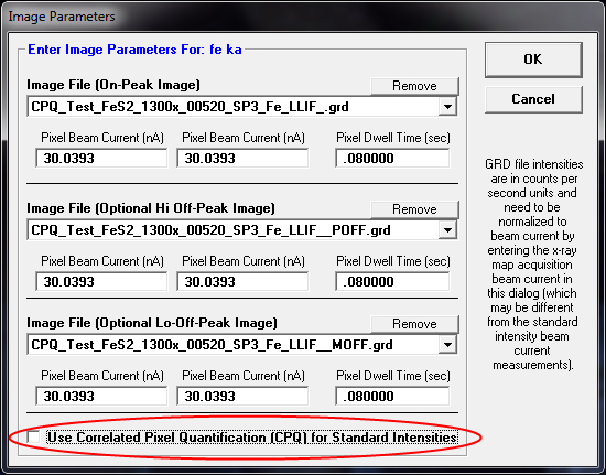
Clearly we have a severe Bragg defocusing problem. However, let's also acquire the same set of maps on our Fe standard (pure Fe) and S standard (also FeS2) and apply them as seen here in CalcImage by clicking on each element and checking the Use Correlated Pixel Quantification check box seen here:
Then we simply load in our standard intensity maps (note that the off-peak intensity maps shown here aren't really necessary in practice as pointed out earlier) into the primary standard locations using the Browse buttons:
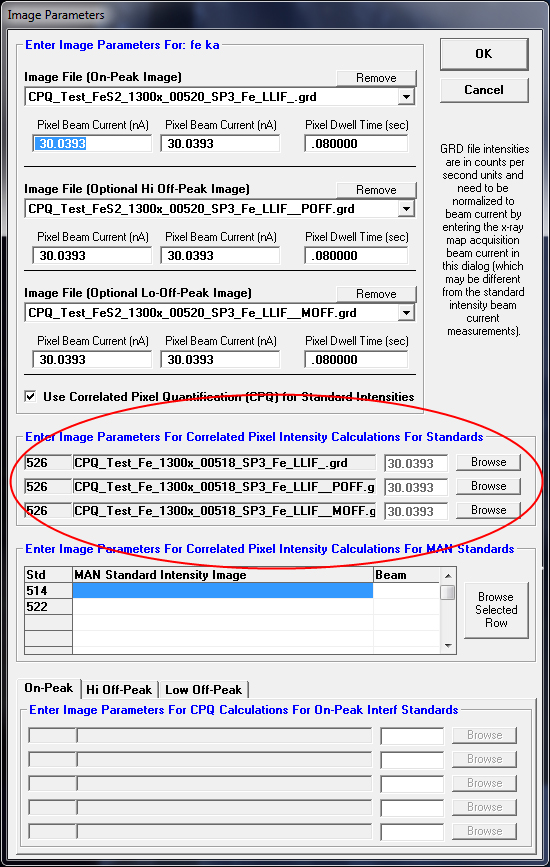
Note that one can also specify MAN standard maps and also interference standard intensity x-ray maps for the primary intensities if the analytical situation requires them.
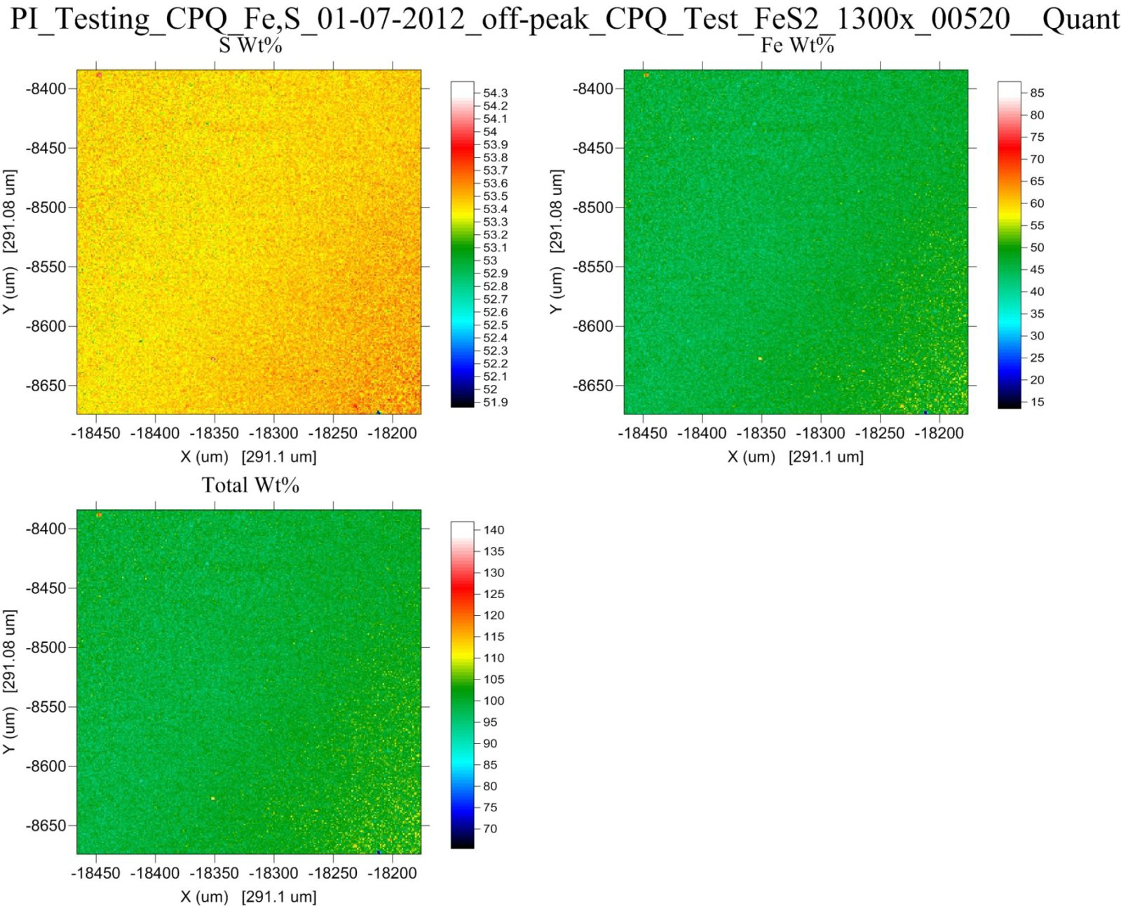
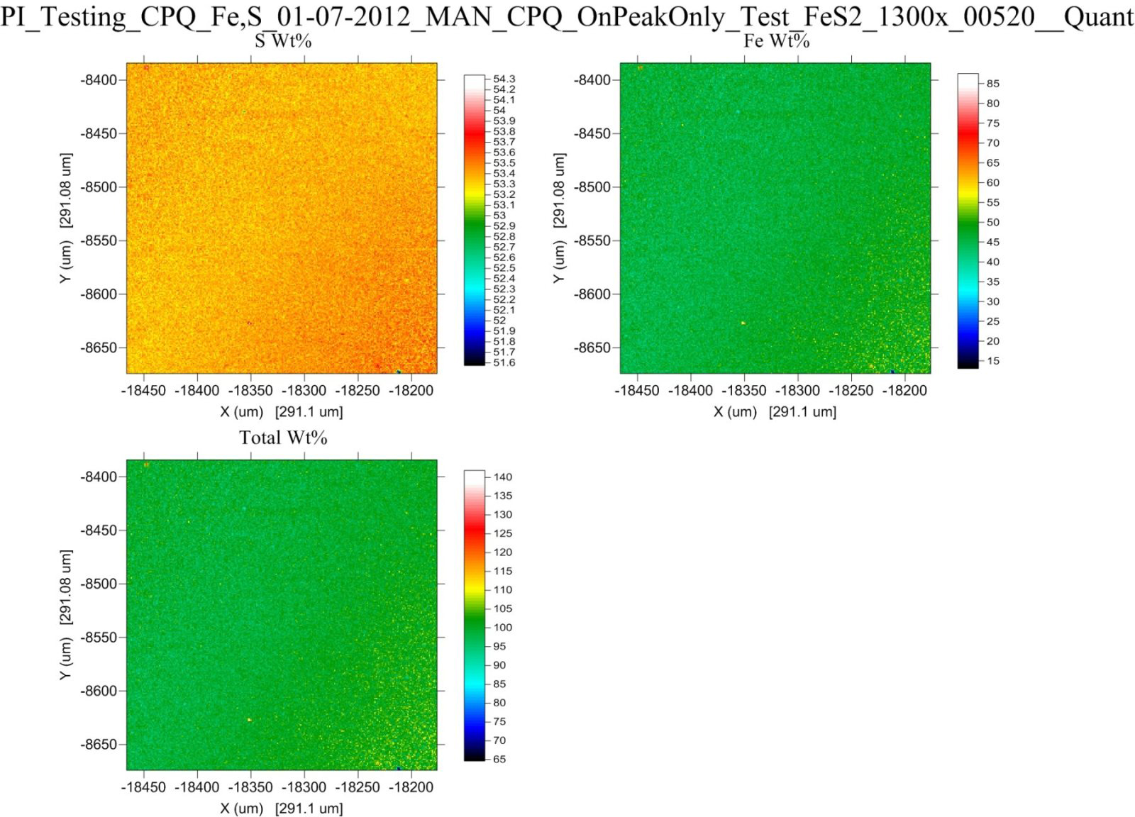
We then perform the same assignments for the S Ka standard x-ray maps and because we have captured the WDS Bragg defocusing effect on both our standard and unknown in the same manner, the k-ratio calculated from the correlated pixels from the unknown and standard x-ray maps nicely corrects for the Bragg defocusing to the level of precision with which the maps were acquired.
Note that at the most extreme Bragg defocusing in some "corners" of the maps, the precision is clearly reduced.
By the way, the same calculation can be performed using MAN backgrounds so that no off-peak maps need be acquired at all as seen here:
Can you tell them apart? It's not easy! Remember, Bragg defocusing mainly affects the characteristic peaks!


 To post in-line images, login and click on the Gallery link at the top