Author Topic: Tips and Tricks for PFE quant  (Read 28076 times)

Probeman

  • Emeritus
  • *****
  • Posts: 2836
  • Never sleeps...
    • John Donovan
Re: Tips and Tricks for PFE quant
« Reply #15 on: November 03, 2016, 09:03:22 AM »
So I investigated further the previously mentioned issue where I got different relative errors on the Si Ka in HfSiO4 when using the empirically measured MAC for Si ka in Hf and found the reason. Unfortunately I do understand the physics of the reason. I even ran this by Paul Carpenter earlier this week, but he was stumped as well. Maybe some of you can enlighten us on what exactly is going on here, because it sure seems unintuitive.  But that's physics for you!

Ok, I made a new short run of ZrSiO4 as the Si standard and HfSiO4 as the Hf standard (oxygen by specification), so let's start by comparing the analysis of Si Ka in HfSiO4 using Hf La and 20 keV beam (just to make things difficult). Here is the analysis of HfSiO4 using the default Henke MACs (without the empirically measured MAC for Si Ka in Hf):

ELEM:       Zr      Hf      Si       O   SUM 
   101    .016  66.589  15.174  23.653 105.431
   102    .038  66.616  15.214  23.653 105.522
   103    .049  66.556  15.096  23.653 105.354

AVER:     .034  66.587  15.161  23.653 105.436
SDEV:     .017    .030    .060    .000    .084
SERR:     .010    .017    .035    .000
%RSD:    49.46     .04     .40     .00

PUBL:     n.a.  65.967  10.380  23.653 100.000
%VAR:      ---   (.94)   46.06     .00
DIFF:      ---   (.62)   4.781    .000
STDS:      257      19     257     ---

STKF:    .4109   .5749   .1274     ---
STCT:   4248.7 14759.3   787.7     ---

UNKF:    .0002   .5749   .0554     ---
UNCT:      1.7 14759.3   342.6     ---
UNBG:      9.1   243.1     3.8     ---

ZCOR:   2.0923  1.1581  2.7362     ---
KRAW:    .0004  1.0000   .4350     ---
PKBG:     1.19   61.73   91.83     ---

Yes, nasty. And remember, the default Armstrong phi-rho-z gave the *worst* correction of all 10 matrix corrections in PFE, but don't worry about that for now.

And here for the record are the Henke MACs that were utilized:

Current Mass Absorption Coefficients From:
LINEMU   Henke (LBL, 1985) < 10KeV / CITZMU > 10KeV

  Z-LINE   X-RAY Z-ABSOR     MAC
      Zr      la      Zr  7.7749e+02
      Zr      la      Hf  3.6888e+03
      Zr      la      Si  2.6349e+03
      Zr      la      Co  1.6648e+03
      Zr      la      O   6.6065e+02
      Hf      la      Zr  1.3762e+02
      Hf      la      Hf  1.7099e+02
      Hf      la      Si  6.3939e+01
      Hf      la      Co  3.3125e+02
      Hf      la      O   1.1692e+01
      Si      ka      Zr  1.1459e+03
      Si      ka      Hf  5.4492e+03
      Si      ka      Si  3.5048e+02
      Si      ka      Co  2.5192e+03
      Si      ka      O   1.0337e+03

The ones in red are the MACs that matter for measuring Si Ka in HfSiO4.  Now the same thing but using the FFAST MACs from NIST:

ELEM:       Zr      Hf      Si       O   SUM 
   101    .015  66.515  14.480  23.653 104.664
   102    .036  66.543  14.519  23.653 104.752
   103    .046  66.483  14.406  23.653 104.589

AVER:     .033  66.514  14.469  23.653 104.668
SDEV:     .016    .030    .058    .000    .082
SERR:     .009    .017    .033    .000
%RSD:    49.46     .04     .40     .00

PUBL:     n.a.  65.967  10.380  23.653 100.000
%VAR:      ---   (.83)   39.39     .00
DIFF:      ---   (.55)   4.088    .000
STDS:      257      19     257     ---

STKF:    .4045   .5730   .1304     ---
STCT:   4248.7 14759.3   787.7     ---

UNKF:    .0002   .5730   .0567     ---
UNCT:      1.7 14759.3   342.6     ---
UNBG:      9.1   243.1     3.8     ---

ZCOR:   2.0185  1.1608  2.5500     ---
KRAW:    .0004  1.0000   .4350     ---
PKBG:     1.19   61.73   91.83     ---

Better, but still pretty bad. And here are the FFAST MACs:

Current Mass Absorption Coefficients From:
FFAST    Chantler (NIST v 2.1, 2005)

  Z-LINE   X-RAY Z-ABSOR     MAC
      Zr      la      Zr  6.9520e+02
      Zr      la      Hf  3.3049e+03
      Zr      la      Si  2.6600e+03
      Zr      la      Co  1.5860e+03
      Zr      la      O   6.2295e+02
      Hf      la      Zr  1.3390e+02
      Hf      la      Hf  1.5115e+02
      Hf      la      Si  6.4790e+01
      Hf      la      Co  3.3857e+02
      Hf      la      O   1.1053e+01
      Si      ka      Zr  1.0291e+03
      Si      ka      Hf  4.9269e+03
      Si      ka      Si  3.2280e+02
      Si      ka      Co  2.4047e+03
      Si      ka      O   9.6997e+02

So far so good as this makes sense to me because the FFAST MACs for Si ka in Hf (and O) are both lower than the Henke MACs, so we expect the Si concentration to be lower, correct?
The only stupid question is the one not asked!

Probeman

  • Emeritus
  • *****
  • Posts: 2836
  • Never sleeps...
    • John Donovan
Re: Tips and Tricks for PFE quant
« Reply #16 on: November 03, 2016, 09:12:10 AM »
Now, let try the same thing, but this time we'll use the empirically measured MAC for Si Ka in Hf, and the other MACs from the Henke or FFAST look up tables.

So here is the analysis using Henke MACs:

ELEM:       Zr      Hf      Si       O   SUM 
   101    .016  66.057  11.044  23.653 100.770
   102    .038  66.083  11.075  23.653 100.850
   103    .049  66.027  10.986  23.653 100.715

AVER:     .034  66.056  11.035  23.653 100.778
SDEV:     .017    .028    .045    .000    .068
SERR:     .010    .016    .026    .000
%RSD:    49.46     .04     .41     .00

PUBL:     n.a.  65.967  10.380  23.653 100.000
%VAR:      ---   (.14)    6.31     .00
DIFF:      ---   (.09)    .655    .000
STDS:      257      19     257     ---

STKF:    .4109   .5749   .1274     ---
STCT:   4248.7 14759.3   787.7     ---

UNKF:    .0002   .5749   .0554     ---
UNCT:      1.7 14759.3   342.6     ---
UNBG:      9.1   243.1     3.8     ---

ZCOR:   2.0881  1.1489  1.9915     ---
KRAW:    .0004  1.0000   .4350     ---
PKBG:     1.19   61.73   91.83     ---

So that is when we see the ~6% relative accuracy error. And here are the MACs utilized:

Current Mass Absorption Coefficients From:
LINEMU   Henke (LBL, 1985) < 10KeV / CITZMU > 10KeV

  Z-LINE   X-RAY Z-ABSOR     MAC
      Zr      la      Zr  7.7749e+02
      Zr      la      Hf  3.6888e+03
      Zr      la      Si  2.6349e+03
      Zr      la      Co  1.6648e+03
      Zr      la      O   6.6065e+02
      Hf      la      Zr  1.3762e+02
      Hf      la      Hf  1.7099e+02
      Hf      la      Si  6.3939e+01
      Hf      la      Co  3.3125e+02
      Hf      la      O   1.1692e+01
      Si      ka      Zr  1.1459e+03
      Si      ka      Hf  3.4770e+03 *
      Si      ka      Si  3.5048e+02
      Si      ka      Co  2.5192e+03
      Si      ka      O   1.0337e+03
 * indicates empirical MAC

Empirical Mass Absorption Coefficients From:
C:\ProgramData\Probe Software\Probe for EPMA\EMPMAC.DAT

  Z-LINE   X-RAY Z-ABSOR     MAC
      Si      ka      Hf  3.4770e+03    Donovan (2011)

Now, the same thing but this time we use the FFAST MACs:

ELEM:       Zr      Hf      Si       O   SUM 
   101    .015  66.104  11.368  23.653 101.140
   102    .036  66.130  11.400  23.653 101.220
   103    .046  66.073  11.309  23.653 101.081

AVER:     .032  66.103  11.359  23.653 101.147
SDEV:     .016    .029    .046    .000    .069
SERR:     .009    .017    .027    .000
%RSD:    49.46     .04     .41     .00

PUBL:     n.a.  65.967  10.380  23.653 100.000
%VAR:      ---   (.21)    9.43     .00
DIFF:      ---   (.14)    .979    .000
STDS:      257      19     257     ---

STKF:    .4045   .5730   .1304     ---
STCT:   4248.7 14759.3   787.7     ---

UNKF:    .0002   .5730   .0567     ---
UNCT:      1.7 14759.3   342.6     ---
UNBG:      9.1   243.1     3.8     ---

ZCOR:   2.0107  1.1536  2.0019     ---
KRAW:    .0004  1.0000   .4350     ---
PKBG:     1.19   61.73   91.83     ---

Ok, so there's the ~9% relative error I was seeing. And here are the MACs utilized:

Current Mass Absorption Coefficients From:
FFAST    Chantler (NIST v 2.1, 2005)

  Z-LINE   X-RAY Z-ABSOR     MAC
      Zr      la      Zr  6.9520e+02
      Zr      la      Hf  3.3049e+03
      Zr      la      Si  2.6600e+03
      Zr      la      Co  1.5860e+03
      Zr      la      O   6.2295e+02
      Hf      la      Zr  1.3390e+02
      Hf      la      Hf  1.5115e+02
      Hf      la      Si  6.4790e+01
      Hf      la      Co  3.3857e+02
      Hf      la      O   1.1053e+01
      Si      ka      Zr  1.0291e+03
      Si      ka      Hf  3.4770e+03 *
      Si      ka      Si  3.2280e+02
      Si      ka      Co  2.4047e+03
      Si      ka      O   9.6997e+02
 * indicates empirical MAC

Empirical Mass Absorption Coefficients From:
C:\ProgramData\Probe Software\Probe for EPMA\EMPMAC.DAT

  Z-LINE   X-RAY Z-ABSOR     MAC
      Si      ka      Hf  3.4770e+03    Donovan (2011)

Ok, so here is the question I have:  why is the concentration so much different when the only difference is the Si Ka in oxygen MAC, and even more weird, why is the Si concentration *higher* in the FFAST calculation, when the Si Ka in O FFAST MAC is *lower* than the Henke MAC value!

 :o
« Last Edit: November 03, 2016, 10:21:08 AM by Probeman »
The only stupid question is the one not asked!

Probeman

  • Emeritus
  • *****
  • Posts: 2836
  • Never sleeps...
    • John Donovan
Re: Tips and Tricks for PFE quant
« Reply #17 on: November 03, 2016, 10:18:33 AM »
In summary here are the results for all 10 analytical expressions using the Henke MACs (and the empirically measured MAC for Si ka in Hf):

Summary of All Calculated (averaged) Matrix Corrections:
St   19 Set   1 HfSiO4 (Hafnon)
LINEMU   Henke (LBL, 1985) < 10KeV / CITZMU > 10KeV

Elemental Weight Percents:
ELEM:       Zr      Hf      Si       O   TOTAL
     1    .034  66.056  11.035  23.653 100.778   Armstrong/Love Scott (default)
     2    .030  65.896   9.987  23.653  99.566   Conventional Philibert/Duncumb-Reed
     3    .031  65.923  10.038  23.653  99.645   Heinrich/Duncumb-Reed
     4    .031  65.939  10.192  23.653  99.816   Love-Scott I
     5    .032  65.946  10.237  23.653  99.868   Love-Scott II
     6    .030  65.878   9.852  23.653  99.414   Packwood Phi(pz) (EPQ-91)
     7    .034  65.993  10.943  23.653 100.622   Bastin (original) Phi(pz)
     8    .033  66.008  10.640  23.653 100.334   Bastin PROZA Phi(pz) (EPQ-91)
     9    .031  65.955  10.275  23.653  99.914   Pouchou and Pichoir-Full (Original)
    10    .031  65.924  10.069  23.653  99.676   Pouchou and Pichoir-Simplified (XPP)

AVER:     .032  65.952  10.327  23.653  99.963
SDEV:     .001    .054    .408    .000    .461
SERR:     .000    .017    .129    .000

MIN:      .030  65.878   9.852  23.653  99.414
MAX:      .034  66.056  11.035  23.653 100.778

And here are the results for all 10 analytical expressions using the FFAST MACs (and the empirically measured MAC for Si ka in Hf):

Summary of All Calculated (averaged) Matrix Corrections:
St   19 Set   1 HfSiO4 (Hafnon)
FFAST    Chantler (NIST v 2.1, 2005)

Elemental Weight Percents:
ELEM:       Zr      Hf      Si       O   TOTAL
     1    .032  66.103  11.359  23.653 101.147   Armstrong/Love Scott (default)
     2    .028  65.953  10.284  23.653  99.919   Conventional Philibert/Duncumb-Reed
     3    .029  65.960  10.333  23.653  99.976   Heinrich/Duncumb-Reed
     4    .030  65.982  10.488  23.653 100.153   Love-Scott I
     5    .030  65.988  10.538  23.653 100.210   Love-Scott II
     6    .029  65.922  10.126  23.653  99.731   Packwood Phi(pz) (EPQ-91)
     7    .032  66.012  11.270  23.653 100.967   Bastin (original) Phi(pz)
     8    .031  66.059  10.968  23.653 100.711   Bastin PROZA Phi(pz) (EPQ-91)
     9    .030  66.002  10.578  23.653 100.263   Pouchou and Pichoir-Full (Original)
    10    .029  65.969  10.363  23.653 100.014   Pouchou and Pichoir-Simplified (XPP)

AVER:     .030  65.995  10.631  23.653 100.309
SDEV:     .001    .053    .424    .000    .473
SERR:     .000    .017    .134    .000

MIN:      .028  65.922  10.126  23.653  99.731
MAX:      .032  66.103  11.359  23.653 101.147

Please note that the correct value for Si in HfSiO4 should be close to 10.38 wt.%...

By the way, I did have a thought (dangerous I know), that perhaps it's the standard k-factor calculation for Si ka in the Si standard which is ZrSiO4. Note that the value for Si Ka in Zr is quite large for both, as seen here:

Henke:
Si      ka      Zr  1.1459e+03

FFAST:
Si      ka      Zr  1.0291e+03

and in fact are some 10 or 11% different.  But more interesting is that the FFAST value is lower, which in the standard, could push the calculated analysis for Si in the unknown (the HfSiO4) in the opposite direction...  so maybe that's the answer?

I've attached the MDB file below is anyone wants to play with it.  If you don't have PFE and just CalcZAF, I've also attached a CalcZAF input file...
« Last Edit: November 03, 2016, 12:42:41 PM by Probeman »
The only stupid question is the one not asked!

Probeman

  • Emeritus
  • *****
  • Posts: 2836
  • Never sleeps...
    • John Donovan
Re: Tips and Tricks for PFE quant
« Reply #18 on: January 22, 2017, 11:19:08 AM »
I think I've mentioned this previously, but I thought I should point out that any data type that is displayed in the PFE Analyze! window, can also be exported directly to Excel by first opening a link to Excel using the Output | Open Link To Excel menu, then by clicking the >>Excel button in Analyze! as seen here:


john
« Last Edit: April 12, 2020, 06:53:34 PM by John Donovan »
The only stupid question is the one not asked!

Probeman

  • Emeritus
  • *****
  • Posts: 2836
  • Never sleeps...
    • John Donovan
Re: Tips and Tricks for PFE quant
« Reply #19 on: March 04, 2017, 10:06:26 AM »
There are often several different ways to design one's analytical approach to a specific sample.  For example, trace element characterization can be approached using various methods contained in Probe for EPMA and it is up to the analyst to decide which approach they deem the best for a particular situation.

For instance, often when I want to measure trace elements in a beam sensitive glass or apatite, my students will often design a "combined condition" analytical setup where the major elements are measured at a low beam current, often using the TDI (time dependent intensity) correction, followed by the trace elements measured at a higher beam current for better sensitivity. An example of this approach is seen here:


Note that both the 30 nA and the 100 nA conditions are contained in the single sample for acquisition and analysis, hence the term "combined condition" sample.  There are other approaches...

Recently a student of Paul Carpenter's wanted to measure trace elements in olivine, so Paul set them up with an analytical method using two separate analytical setups, the first for the major elements at 25 nA, and a second analytical setup at 100 nA (note that Al is acquired on two spectrometers for better sensitivity) as seen here for the 25 nA setup:


and here for the 100 nA setup:


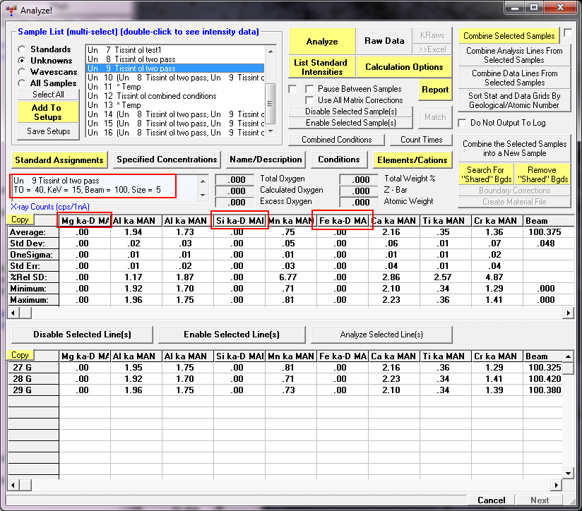
Look closely and you will note that both samples have the same elements! However, the first analytical setup has all the trace elements disabled for acquisition (and quant), and the second analytical setup has all the major elements disabled for acquisition (and quant).  Please note that the disable acquisition and disable quant checkboxes are found in the Elements/Cations dialog for each element.

So, what Paul does is have the student assign *both* analytical setups to each digitized stage coordinate in the Automate! window using the Multiple Setups button. That way the program acquires each analytical setup (with the different beam currents and different elements disabled for acquisition) one after the other.  Once that is done, the user can go to the Analyze! window and combine the elements for the two setups using either of the two buttons highlighted here:


The upper button doesn't permanently combine the data into a new sample, the lower button does permanently combine them. The results for the "combine selected samples" method is shown here:


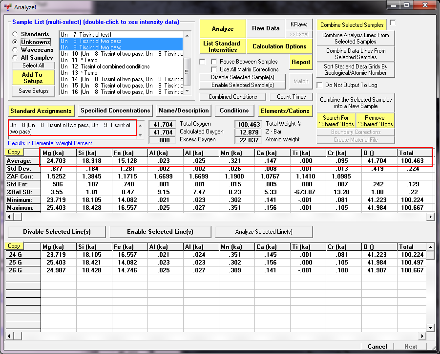
Finally, we can turn on the "aggregate" mode under the Analysis Options dialog and "aggregate" the two aluminum channels for better trace element sensitivity as seen here:

« Last Edit: April 12, 2020, 06:54:07 PM by John Donovan »
The only stupid question is the one not asked!

Probeman

  • Emeritus
  • *****
  • Posts: 2836
  • Never sleeps...
    • John Donovan
Re: Tips and Tricks for PFE quant
« Reply #20 on: March 07, 2017, 05:08:43 PM »
Here's something I ran across today...

I'm running some diffusion profiles in some metallurgical samples and I noticed that my totals were somewhat high around 101.5 wt.% or so.  These are PbS and PbTe samples at 15 keV, so first I checked for interferences, and they are all corrected for properly (one really needs a good Pb standard that doesn't contain S for an interference correction of S Ka on Pb Ma, so I use alamosite or PbSiO3). Then I checked the focus on the unknowns and the standards and that was good too.  No significant intensity drift either.  So why the high totals as seen here? 


Then it occurred to me, the standards are carbon coated, but the unknown is not (the customer doesn't want us to carbon coat their samples, so we've been using Cu tape to ground them to the sample holder). Could that make this much of a difference for Pb Ma and Te La?

So first I went to the Calculation Options dialog in the Analyze! window and unchecked the Use Unknown Conductive Coating as seen here:


Now, if you re-calculate the analysis, one gets the same results, and why is that?   It's because the coatings corrections are not actually utilized in the software unless one specifically turns them on in the Analytical | Analysis Options dialog as seen here:


Now we re-calculate our results and dang if that didn't take care of the high totals:

« Last Edit: April 12, 2020, 06:54:37 PM by John Donovan »
The only stupid question is the one not asked!

John Donovan

  • Administrator
  • Emeritus
  • *****
  • Posts: 3275
  • Other duties as assigned...
    • Probe Software
Re: Tips and Tricks for PFE quant
« Reply #21 on: June 14, 2019, 09:19:05 AM »
This is more of a tip than a trick, but I mention it because we recently improved the Report button output to better handle the presence of elements quantified using the EDS WDS integration feature in Probe for EPMA. The WDS and EDS integration in Probe for EPMA can utilize SDD EDS systems from Thermo (NSS and Pathfinder), Bruker (Esprit) and most recently JEOL (OEM) EDS detectors.

The Report button is located in the Analyze! window as seen here and can be applied to any unknown or standard sample in your run:


This feature can be utilized to export both a text description and a tab delimited spreadsheet format of the current analytical conditions and parameters. The text output consists of (almost!) English sentences as seen here that can be edited for including in your own reports and manuscripts:

Probe for EPMA Xtreme Edition for Electron Probe Micro Analysis
Database File: C:\UserData\Eastman\06-2019\Fe, V, C, O_06-03-2019.MDB
Database File Type: PROBE
DataFile Version Number: 12.6.2
Program Version Number: 12.6.3
Database File User Name: Chris Eastman
Database File Description: C and O by WDS, V, Fe, etc. by EDS

Database Created: 6/3/2019 11:01:40 AM
Last Updated: 6/3/2019 11:01:40 AM
Last Modified: 6/13/2019 1:12:23 PM
Current Date and Time: 6/13/2019 1:13:24 PM
Nominal Beam: 54.2881 (nA)
Faraday/Absorbed Averages: 1

Correction Method and Mass Absorption Coefficient File:
ZAF or Phi-Rho-Z Calculations
LINEMU   Henke (LBL, 1985) < 10KeV / CITZMU > 10KeV

Current ZAF or Phi-Rho-Z Selection:
Armstrong/Love Scott (default)

Correction Selections:
Phi(pz) Absorption of Armstrong/Packwood-Brown 1981 MAS
Stopping Power of Philibert and Tixier
Backscatter Coefficient of Love-Scott
Backscatter of Love-Scott
Mean Ionization of Berger-Seltzer
Phi(pz) Equation of Love-Scott
Reed/JTA w/ M-Line Correction and JTA Intensity Mod.
Fluorescence by Beta Lines NOT Included

Un    2 Fe, V, C, O trav1
TakeOff = 40.0  KiloVolt = 15.0  Beam Current = 30.0  Beam Size =    0
(Magnification (analytical) =  40000),        Beam Mode = Analog  Spot
(Magnification (default) =     2245, Magnification (imaging) =   2857)
Image Shift (X,Y):                                         .00,    .00

Compositional analyses were acquired on an electron microprobe (Cameca SX100/SXFive (TCP/IP Socket)) equipped with 5 tunable wavelength dispersive spectrometers.

EDS spectra were acquired and processed using a Thermo NSS or PF EDS system.

Operating conditions were 40 degrees takeoff angle, and a beam energy of 15 keV.
The beam current was 30 nA, and the beam diameter was 0 microns.

Elements were acquired using analyzing crystals EDS for Fe ka, Nb la, V ka, PC1 for O ka, and PC2 for C ka.

The standards were Carbon (graphite) for C ka, Vanadium metal for V ka, Iron metal for Fe ka, Niobium metal for Nb la, and Al2O3 (elemental) (#13) for O ka.

Iron metal
From Johnson-Matthey, Vacuum remelted, Batch BM1664
Optical emission: Al < 1ppm, Ca < 1 ppm,
Cr 2 ppm, Co 20 ppm, Cu 3 ppm, Ni 3 ppm
Si 60 ppm, Sn 10 ppm, Ag < 1 ppm
Oxygen 310 ppm, Nitrogen 10 ppm

Vanadium metal
From Aesar, #143594, Lot #19778
99.95%, 1.0 mm wire

Carbon (graphite)
1. single crystal (synthetic) from Union Carbide
Grade 2YA, serial #8403, contains ~2.4% oxygen (from H2O?)


Al2O3 (elemental) (#13)
Specimen from Baikowski Int'l, North Carolina
'crackle' from seed crystal, 99.99%
Si ~330 PPM by EPMA (JJD), 05-30-2012

Niobium metal
Aesar, 99.99%, 0.25mm sheet
Lot #10258
Possible 0.19 wt% Ta (?)

The counting time was 30 seconds for C ka, O ka, and 45 seconds for Nb la, V ka, Fe ka.

The intensity data was corrected for Time Dependent Intensity (TDI) loss (or gain) using a self calibrated correction for C ka, O ka.

The off peak counting time was 10 seconds for C ka, O ka.

Off Peak correction method was Exponential for C ka, O ka.

Unknown and standard intensities were corrected for deadtime.

Interference corrections were applied to C for interference by Nb, and to O for interference by V, Nb,

See J.J. Donovan, D.A. Snyder and M.L. Rivers, An Improved Interference Correction for Trace Element Analysis in Microbeam Analysis, 2: 23-28, 1993

Results are the average of 10 points and detection limits ranged from .037 weight percent for C ka to .177 weight percent for O ka.

Analytical sensitivity (at the 99% confidence level) ranged from 2.222 percent relative for C ka to 10.142 percent relative for O ka.

The quantitative blank correction was utilized.
The exponential or polynomial background fit was utilized.

See John J. Donovan, Heather A. Lowers and Brian G. Rusk, Improved electron probe microanalysis of trace elements in quartz, American Mineralogist, 96, 274­282, 2011

The matrix correction method was ZAF or Phi-Rho-Z Calculations and the mass absorption coefficients dataset was LINEMU   Henke (LBL, 1985) < 10KeV / CITZMU > 10KeV.

The ZAF or Phi-Rho-Z algorithm utilized was Armstrong/Love Scott (default).

Note the integration of EDS and WDS elements including the ability to apply spectral interference corrections between elements by WDS and EDS.

And here is the tab delimited report format suitable for import to Excel as seen here:


Just FYI.  Available for download now.

Edit by John: In case anyone is wondering why we decided to run O and C by WDS and Fe, V and Nb by EDS, it's a long story, but basically the sample is so magnetic (and re-magnetizes in the instrument), that the Bragg defocus between the standards and unknowns was killing us. So we ran Fe, V and Nb by EDS to avoid the Bragg defocus issue, and ran O and C by WDS because the EDS just can't handle these elements at trace levels. Also because the WDS peaks for O and C are so broad that the Bragg defocus is much less of an issue. The remaining problem now is trying to figure out where the darn beam is/was. Tough problem.
« Last Edit: June 14, 2019, 10:18:57 AM by John Donovan »
John J. Donovan, Pres. 
(541) 343-3400

"Not Absolutely Certain, Yet Reliable"

John Donovan

  • Administrator
  • Emeritus
  • *****
  • Posts: 3275
  • Other duties as assigned...
    • Probe Software
Re: Tips and Tricks for PFE quant
« Reply #22 on: December 06, 2019, 10:00:01 AM »
Here's another tip for those working with unusual compositions and wanting to classify those compositions and their modal abundances.

Normally for modal calculations of common silicates and oxides one can utilize the DHZ.MDB standard composition database because it contains most common rock forming minerals. But when working with unusual compositions, one should consider creating their own "custom" standard database (custom.mdb) for modal calculations.

One way to do this (other than simply entering the compositions by hand into the custom.mdb file), is when you are in the Analyze! window and have an analysis displayed, to simply right click the analyzed sample and click the Export Selected Samples To Custom.MDB menu.


The Probe for EPMA software will then export the average composition of each sample to the custom.mdb standard database, which can then be used on your quantitative WDS maps for modal identification in the CalcImage software as described here:

https://probesoftware.com/smf/index.php?topic=1071.msg7095#msg7095
John J. Donovan, Pres. 
(541) 343-3400

"Not Absolutely Certain, Yet Reliable"

alerner

  • Graduate
  • **
  • Posts: 6
Re: Tips and Tricks for PFE quant
« Reply #23 on: February 05, 2020, 04:57:52 PM »
Hi all,

A useful approach that I've been using to assess the quality of standard analyses (unknowns too) within the Analyze! window is to use the String Selection field to search for and highlight all instances of a particular standard across multiple standard sets (where * can be used as a wildcard), and then output all these analyses with "Combine Data Lines from Selected Samples". This results in a easy to view output of all standards run for that entire session, so that the intensity reproducibility and/or drift with time can be seen. It is then easy to Disable anomalous measurements from within the data display.

I follow suite with particular sets of unknowns of interest, and "Combine Analysis Lines from Selected Samples" to easily view the output data + assess totals.


Best,
Allan Lerner
« Last Edit: February 06, 2020, 08:30:30 AM by John Donovan »

John Donovan

  • Administrator
  • Emeritus
  • *****
  • Posts: 3275
  • Other duties as assigned...
    • Probe Software
Re: Tips and Tricks for PFE quant
« Reply #24 on: November 10, 2021, 08:47:27 AM »
Just to add to Alan's point above, the latest version of Probe for EPMA now allows one to combine data lines from 2 or more samples (up to 500 lines total) now including the EDS spectra elements as well:


In the above example, the elements Mg, K and Fe were acquired by EDS for quantification. This is seen in the following screenshot with the same samples combined and just displaying the intensities:


Thanks to Scott Boroughs for calling attention to a bug when including the quant EDS elements that is now fixed.
John J. Donovan, Pres. 
(541) 343-3400

"Not Absolutely Certain, Yet Reliable"

Rom

  • Professor
  • ****
  • Posts: 152
Re: Tips and Tricks for PFE quant
« Reply #25 on: January 27, 2022, 04:08:43 AM »
Hi everyone,
could you explain how I can use options "standard X increment, ..." only for some standards of my "Run", not for all standards which will measure.
Thank you.

Probeman

  • Emeritus
  • *****
  • Posts: 2836
  • Never sleeps...
    • John Donovan
Re: Tips and Tricks for PFE quant
« Reply #26 on: January 27, 2022, 08:28:43 AM »
Digitize the standard positions exactly as you want them in the Automate! window, then in Acquisition Options check the checkbox "Use Only Digitized Standard Positions".

See also:

https://probesoftware.com/smf/index.php?topic=8.msg4011#msg4011
The only stupid question is the one not asked!

Rom

  • Professor
  • ****
  • Posts: 152
Re: Tips and Tricks for PFE quant
« Reply #27 on: January 27, 2022, 03:43:55 PM »
The option "acquire standard samples (again)" work at this way, but the points positions on the second, third, ... run will be the same - am I right?
Or checkbox "re-standard Y increment" will work?

Probeman

  • Emeritus
  • *****
  • Posts: 2836
  • Never sleeps...
    • John Donovan
Re: Tips and Tricks for PFE quant
« Reply #28 on: January 27, 2022, 03:57:36 PM »
Easy enough to test it, but yes, re-standard increment in Y still applies for standards.
The only stupid question is the one not asked!

Rom

  • Professor
  • ****
  • Posts: 152
Re: Tips and Tricks for PFE quant
« Reply #29 on: January 27, 2022, 04:06:46 PM »
Thank you!