Limits of detection and precision for quantitative maps

[AndrewLocock]

I wanted to inquire about the limits of detection and estimated precision for quantitative WDS mapping.
Am I right in thinking that they will be considerably worse than a typical spot analysis, because of the large difference in acquisition time?

I am only considering the effects of X-ray counting statistics.
For example, a spot analysis run under typical conditions (15 kV, 20 nA, focussed beam, 20 seconds on peak) might have a detection limit of 100 ppm for some element.

If a map of this element is run at the same column conditions, but the dwell time on a pixel is 200 milliseconds (a factor of 100 less acquisition time), then I would expect the limit of detection for that element to be 1000 ppm (10 times higher: square root of 100) for the pixel in the map as compared to the spot analysis.

In the past, we have more typically used a 20 millisecond dwell time per pixel (a factor of 1000 less acquisition time compared to the spot analysis), so the detection limit for the pixel in this example would then be about 3162 ppm.

Assuming a similar scaling behavior for precision: a precision of 0.5% for the spot analysis (20 s on peak), becomes 5% for the pixel at 200 millisecond dwell time and almost 16% at 20 millisecond dwell time.

I would be interested to know if this scaling of detection limits and precision is what might be expected during quantitative mapping, given the assumptions listed above.

Thanks,
Andrew

[Probeman]

I would be interested to know if this scaling of detection limits and precision is what might be expected during quantitative mapping, given the assumptions listed above.

Hi Andrew,
I think you are correct.  The precision will increase or decrease with each doubling or halving of the pixel dwell time, by the Sqrt(2).  This of course assumes Gaussian statistics, while x-ray counting is more accurately described by Poisson statistics, but it's close enough and a lot easier to calculate!

Next time you have a chance check the "Calculate Projected Detection Limits" option under Calculation Options in the Analyze! window, and the program will display a range of estimated detection limits based on the counting time of the actual analysis. Here is an example from a synthetic zircon:

Projected Detection Limits (99% CI) in Elemental Weight Percent (Average of Sample):

ELEM:       Th      Hf       U       P       Y
TIME:    10.00   10.00   10.00   10.00   10.00
PROJ:     .035    .028    .031    .007    .048
TIME:    20.00   20.00   20.00   20.00   20.00
PROJ:     .025    .020    .022    .005    .034
TIME:    40.00   40.00   40.00   40.00   40.00
PROJ:     .018    .014    .015    .003    .024
TIME:    80.00   80.00   80.00   80.00   80.00
PROJ:     .012    .010    .011    .002    .017
TIME:   160.00  160.00  160.00  160.00  160.00
PROJ:     .009    .007    .008    .002    .012
TIME:   320.00  320.00  320.00  320.00  320.00
PROJ:     .006    .005    .005    .001    .008
TIME:   640.00  640.00  640.00  640.00  640.00
PROJ:     .004    .003    .004    .001    .006
TIME:  1280.00 1280.00 1280.00 1280.00 1280.00
PROJ:     .003    .002    .003    .001    .004
TIME:  2560.00 2560.00 2560.00 2560.00 2560.00
PROJ:     .002    .002    .002    .000    .003
TIME:  5120.00 5120.00 5120.00 5120.00 5120.00
PROJ:     .002    .001    .001    .000    .002
TIME: 10240.0010240.0010240.0010240.0010240.00
PROJ:     .001    .001    .001    .000    .001
TIME: 20480.0020480.0020480.0020480.0020480.00
PROJ:     .001    .001    .001    .000    .001
TIME: 40960.0040960.0040960.0040960.0040960.00
PROJ:     .001    .000    .000    .000    .001

The bolded lines are the actual acquisition time.

This sensitivity limitation for x-ray mapping due to (humanly) reasonable dwell times per pixel, is also a reason why the blank correction, which is normally in the sub 50 PPM range, is not necessary when performing most x-ray mapping as seen here, where the on-peak dwell time per pixel is only 3 seconds:

http://probesoftware.com/smf/index.php?topic=42.msg4813#msg4813

Yes, with a single point analysis we can acquire for hundreds of seconds per point (e.g., my claim of 2-3 PPM of Ti in quartz in Donovan et al., Amer. Min., 2011 using 5 spectrometers aggregated), but a 128 x 128 pixel map consisting of 300 seconds per pixel would take 1365 hours or 56 days!

It would be a gorgeous map though.   I did something similar a few years ago by acquiring a grid of point analyses on a quartz from Butte, MN, using Probe for EPMA with some 400 points and after Kriging the data in Surfer I got a map like this after about a week of acquisition:



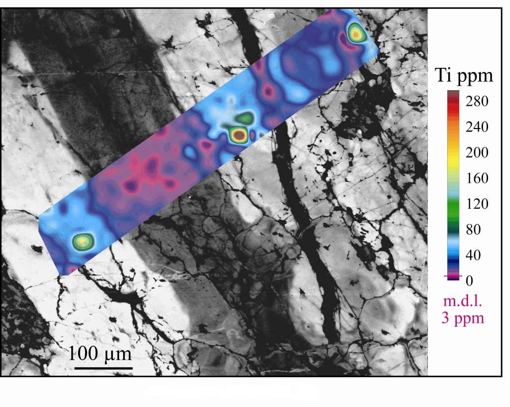
This image is a figure from the above mentioned Amer. Min. paper.
john

[Ben Buse]

Hi Andrew,

Yes you're right. I guess the only other things to point out is although x-ray maps have very short count times, they are typically run at much higher beam currents to recover some of the precision. And secondly where features are large e.g. a elongate zone you can see variations in intensity which would not be detectable from a single point. It's a question of signal to noise ratio and your eye can blur pixels. You can also draw wide line scans on maps which sum pixels

Just a note, you may be doing this, to be strictly correct the ratio of peak to background is important not just square root when calculating errors/detection limits. Particularly at low concentration. This can be done using the equations for each pixel in a map. Or instead of putting the equations in Excel you can also use the detection limit calculator in Calczaf.

Ben

[Probeman]

Just a note, you may be doing this, to be strictly correct the ratio of peak to background is important not just square root when calculating errors/detection limits. Particularly at low concentration. This can be done using the equations for each pixel in a map. Or instead of putting the equations in Excel you can also use the detection limit calculator in Calczaf.

Hi Ben and Andrew,
One can also just check the "Output Detection Limits" option in CalcImage to get a pixel by pixel detection limit map as seen here:



These values are calculated using the Goldstein et al. method of 3 times the Sqrt(background intensity) divided by the standard intensity and matrix corrected as described in the PFE help file. Note that the detection limit can vary quite a bit depending on the specific matrix.
john

[Probeman]

Another reason for performing fully quant maps is that the raw data can be deceiving depending on the matrix effects.

Here are two oxygen maps from Anette von der Handt. Not sure what the exact matrix was, but the first map is the raw (qualitative) map which is traditionally utilized:



And here is the background, matrix and interference corrected x-ray map acquired with Probe Image and quantified by CalcImage:



Imagine reporting our single point analyses in raw cps... it should be no different for x-ray maps- if we want to accurately interpret our map data!

[Probeman]

... And secondly where features are large e.g. a elongate zone you can see variations in intensity which would not be detectable from a single point. It's a question of signal to noise ratio and your eye can blur pixels.

Here's an example of what Ben is talking about, where the eye can pick out subtle differences that are not statistically significant (see the last several images of trace Mo maps in pyrite and chalcopyrite phases):

http://probesoftware.com/smf/index.php?topic=708.msg4367#msg4367

In the interference corrected Mo map, one can see a subtle difference, though the averages of the two phases are not statistically different...

[Probeman]

I wanted to inquire about the limits of detection and estimated precision for quantitative WDS mapping.

Hi Andrew,
I should also point out that you can also easily generate analytical sensitivity maps along with your quant x-ray maps as seen here:

http://probesoftware.com/smf/index.php?topic=652.msg3862#msg3862

Remember you need to be logged in to see these attachments.

And unlike detection limits which are in elemental wt.%, the analytical sensitivity maps are in relative percent error (1 sigma) units.
john

[Probeman]

I'll try and find a better example because it's a little hard to see, but here's a different kind of difference between raw data and quant x-ray maps, than what we saw in Anette's oxygen x-maps above where the matrix correction dominates. In these maps, the map on the left are the on-peak intensities for oxygen in a Fe-Ni-Cr alloy. On the right is the wt. % quant map of oxygen.

The interesting thing is that the two major phases that show higher trace oxygen are exactly opposite in the raw vs. quant x-ray maps. The reason being that traces are more accurately interpreted once a proper background correction has been applied.



Can everyone see the opposite trends in the two phases?  Does anyone have a better example?

[Probeman]

With regard to detection limits, here's a slightly better example from the Mo in pyrite/chalcopyrite interference x-ray maps I showed earlier this summer:

http://probesoftware.com/smf/index.php?topic=708.msg4367#msg4367

But this time we are looking at the Zn Ka signal. On the left you see the raw Zn Ka map, and on the right the quantified x-ray map (background, matrix, etc corrected):



In the raw intensity map on the left one might think there were two different concentrations of Zn in the pyrite vs. the chalcopyrite, So is this difference due to an interference on Zn Ka?  No. In fact the levels in the quantified map are about the same after the map is corrected for background.