Quant Analysis of Carbon Using MAN backgrounds

[John Donovan]

I attempted some C ka measurements in my transition element stds and the results are promising. Here's the MAN fit:



There were some interferences from the light elements (Mg and Al) so I left them out of the MAN bgd calibration. The Cu std also gave a bad interference so that was left out of the bgd fit also.  Note that on-peak interferences can be corrected for using the PFE interference correction if the interfering element is also measured. Otherwise just avoid that interference in the MAN calibration curve.

The spot analyses on Fe are here:

ELEM:        C      Fe   SUM 
   241   -.010 100.439 100.429
   242   -.036  99.932  99.896
   243   -.019  99.570  99.551
   244    .022 100.490 100.511
   245   -.019  99.528  99.509

AVER:    -.012  99.992  99.979
SDEV:     .021    .460    .474
SERR:     .010    .206
%RSD:  -172.15     .46

PUBL:     n.a. 100.000 100.000
%VAR:      ---  (-.01)
DIFF:      ---  (-.01)
STDS:      506     526

So 120 PPM +/- 210 PPM is not too bad!

Here is Cr metal using the same calibration curve:

ELEM:        C      Fe   SUM 
   231    .008   -.007 100.001
   232    .019    .055 100.073
   233    .017   -.036  99.981
   234   -.015    .043 100.029
   235    .017    .048 100.065

AVER:     .009    .020 100.030
SDEV:     .014    .040    .040
SERR:     .006    .018
%RSD:   155.63  195.90

PUBL:     n.a.    .010 100.010
%VAR:      ---  104.79
DIFF:      ---    .010
STDS:      506     526

And here is the Ni std, again using the same calibration curve:

ELEM:        C      Fe   SUM 
   251    .020    .073 100.093
   252    .028    .027 100.055
   253    .041   -.006 100.035
   254    .000    .007 100.006
   255    .031   -.025 100.006

AVER:     .024    .015 100.039
SDEV:     .015    .038    .037
SERR:     .007    .017
%RSD:    64.74  246.91

PUBL:     n.a.    n.a. 100.000
%VAR:      ---     ---
DIFF:      ---     ---
STDS:      506     526

The idea being that one could perform carbon analyses on arbitrary mixtures of alloys.
john

PS These analyses were performed at 10 keV, 30 nA and a 40 sec count time for C ka (on-peak only).

Sensitivity of around 200 PPM is pretty impressive for a diffusion pumped (and cryo-baffle cooled) vacuum system!

[John Donovan]

First attempt at a 1 pixel high line beam scan using MAN backgrounds for carbon ka showing the effect of the beam intercepting the carbon contamination ring around the initial beam position.
john

[John Donovan]

Question to all:

is the small initial decrease in carbon concentration on the left side of the graph from the 0.1 % level to zero an indication of the desorption of the "native" carbon layer as the sample heats up during the first 3 or 4 steps (all within 300 or 400 nm (15 to 20 secs) of each other)?

In other words is this what the Aachen lab means when they describe the need for an initial "decontamination time"?

[John Donovan]

Here's another carbon (and now also nitrogen!) measurement in steel using an MAN background fit for carbon and nitrogen, both without and with a blank correction on a vacuum remelted Fe metal standard (O 310 ppm, N 10 ppm, C assumed 0 PPM).

First here are the MAN fits for carbon (PC2 crystal):



and for nitrogen (PC1 crystal):



and here are the quantitative plots without the blank correction applied to carbon and nitrogen:



Note that the nitrogen values fall off the bottom of the scale because without the blank correction, the values are a few hundred PPM negative (and cannot be plotted on a log scale), basically the limit of accuracy for the MAN correction.

And now with the blank correction applied to the MAN bgd correction:



Note that the nitrogen values now approach zero (as they should).

This MAN background correction is very similar to the EU ISO method, except that we utilize several standards for the continuum fit model to deal with changes in average atomic number in the sample (up to 7 wt% N and 4 % C which yields an average atomic number of approximately 24.3 as opposed to pure Fe which is of course, around 26).

The Analyze! window Report button generates the following English sentences about the sample:

Compositional analyses were acquired on an electron microprobe (Cameca SX100 (TCP/IP Socket)) equipped with 5 tunable wavelength dispersive spectrometers. Operating conditions were 40 degrees takeoff angle, and a beam energy of 10 keV.  The beam current was 50 nA, and the beam diameter was 0 microns.

Elements were acquired using analyzing crystals LIF for Fe ka, Mn ka, Ni ka, Cu ka, LPET for Mo la, Cr ka, LTAP for Al ka, Si ka, PC1 for N ka, and PC2 for C ka.

The standards were Carbon (graphite) for C ka, Aluminum metal for Al ka, Silicon metal for Si ka, Chromium metal for Cr ka, Manganese metal for Mn ka, Iron metal for Fe ka, Nickel metal for Ni ka, Copper metal for Cu ka, Molybedenum metal for Mo la, and AlN ceramic for N ka.

The counting time was 20 seconds for Fe ka, 40 seconds for Mn ka, Ni ka, Cu ka, 60 seconds for C ka, N ka, and 80 seconds for Mo la, Cr ka, Al ka, Si ka.  The off peak counting time was 6 seconds for Fe ka, 20 seconds for Mn ka, Ni ka, Cu ka, and 40 seconds for Mo la, Cr ka, Al ka, Si ka.  Off Peak correction method was Linear for Mo la, Cr ka, Fe ka, Mn ka, Ni ka, Cu ka, and Exponential for Al ka, Si ka.

The MAN background intensity data was calibrated and continuum absorption corrected for C ka, N ka.  See J.J. Donovan and T.N. Tingle, An Improved Mean Atomic Number Correction for  Quantitative Microanalysis in Journal of Microscopy, v. 2, 1, p. 1-7, 1996

Unknown and standard intensities were corrected for deadtime. Standard intensities were corrected for standard drift over time.

Interference corrections were applied to C for interference by Cu, and to N for interference by Ni, Cu, and to Fe for interference by Mn, and to Mn for interference by Cr.  See J.J. Donovan, D.A. Snyder and M.L. Rivers, An Improved Interference Correction for Trace Element Analysis in Microbeam Analyis, 2: 23-28, 1993

Results are the average of 139 points and detection limits ranged from .005 weight percent for Si ka to .005 weight percent for Al ka to .030 weight percent for C ka to .214 weight percent for Fe ka to .617 weight percent for Cu ka.

Analytical sensitivity (at the 99% confidence level) ranged from .368 percent relative for Al ka to .519 percent relative for Fe ka to 1.813 percent relative for C ka to 36.425 percent relative for N ka to 398.835 percent relative for Ni ka.

The quantitative blank correction was utilized. The exponential or polynomial background fit was utilized. See John J. Donovan, Heather A. Lowers and Brian G. Rusk, Improved electron probe microanalysis of trace elements in quartz, American Mineralogist, 96, 274

Note: it might be that because all MAN (on-peak) intensity measurements receive the same "induced" carbon contamination rate, the contamination effect gets pretty much "normalized" out between them.  Therefore I found that one should acquire the MAN standards using the same count time as the unknowns (that is, Unknown Count Factors = 1).

[John Donovan]

Here are some more carbon beam scan tests using 0.1 um steps to observe the contamination ring smearing effect I've run recently. I still need to do more measurements at higher currents but...

The first attached jpg is carbon ka on a vacuum remelted Fe std using the normal multi-std MAN background correction with multiple metals for the background fit, and with the "blank" correction turned on to improve the accuracy of the MAN fit. Note the large artifact from the carbon contamination ring "smear" as the beam progressively overlaps onto the previous carbon ring.

The next jpg plot is the same carbon beam scan image with the CPQ correction turned on for the MAN assignment of the iron std only. See here:

http://probesoftware.com/smf/index.php?topic=41.msg178#msg178

for a more complete description of the correlated pixel quantification (CPQ) method. 

I didn't acquire beam scans on the other MAN std metals which means this is equivalent to the Aachen method of only using Fe for the MAN (on-peak) background measurement for carbon ka. Of course the blank correction needs to be turned off in this case. Otherwise, it's as though one is applying the blank correction twice! In the case of carbon about 300 PPM positive (see normal point analyses below).

The CPQ plot is using the carbon ka on Fe std beam scan for both the unknown image and the also for the CPQ std image so ideally the quant data should zero out.  Therefore, this is only a "sanity check" for PFE and CalcImage but still it's nice to see an average very close to zero.

Note the very small 10-20 PPM variance visible in the carbon CPQ plot which I suspect must be due to the differences in the absorption correction from the noise in the iron and nitrogen signals in the beam scan image (carbon ka absorption correction is around 200% in an Fe matrix).
john

Un    2 Fe blank
TakeOff = 40.0  KiloVolt = 10.0  Beam Current = 30.0  Beam Size =    0
(Magnification (analytical) =  40000),        Beam Mode = Analog  Spot
(Magnification (default) =      400, Magnification (imaging) =    800)
Image Shift (X,Y):                                          .00,   .00
Number of Data Lines:   5             Number of 'Good' Data Lines:   4
First/Last Date-Time: 10/24/2013 04:35:53 PM to 10/24/2013 04:42:51 PM
WARNING- Using Blank Trace Correction

Average Total Oxygen:         .000     Average Total Weight%:  100.914
Average Calculated Oxygen:    .000     Average Atomic Number:   26.004
Average Excess Oxygen:        .000     Average Atomic Weight:   55.880
Average ZAF Iteration:        1.00     Average Quant Iterate:     4.00

Un    2 Fe blank, Results in Elemental Weight Percents
 
ELEM:        C      Fe       N
BGDS:      MAN     MAN     MAN
TIME:    80.00   80.00   80.00
BEAM:    30.04   30.04   30.04

ELEM:        C      Fe       N   SUM 
    46    .019 100.613   -.012 100.620
    47    .010 101.488   -.006 101.492
    48    .007 100.472   -.013 100.466
    49    .009 101.174   -.104 101.078

AVER:     .011 100.937   -.034 100.914
SDEV:     .005    .477    .047    .465
SERR:     .003    .238    .024
%RSD:    47.49     .47 -139.79
STDS:      506     526     604

STKF:    .9705  1.0000   .2573
STCT:  1285.92  144.17   14.37

UNKF:    .0000  1.0094  -.0002
UNCT:      .06  145.52    -.01
UNBG:     4.29     .81     .64

ZCOR:   2.4873   .9999  1.5315
KRAW:    .0000  1.0094  -.0009
PKBG:     1.01  181.36     .98
BLNK#:       3    ----       3
BLNKL: .000000    ---- .000000
BLNKV: -.03305    ---- -.28686

And if anyone is wondering how one might  perform such an effective correction for this carbon ring "smearing" effect, provided one acquires a similar image acquisition on the appropriate standard, it really couldn't be easier:

[Probeman]

Analysis of carbon is a special animal...

The first decision one has to make is whether to coat with another material, because generally one doesn't want to coat with the same element as is being analyzed. Al is often used for carbon analysis, but let's look at the mass absorption coefficients (MACs) for carbon Ka in a list of element absorbers. 

Note that Ag is surprisingly good for transmitting C Ka as seen here, especially compared to Al- even though Al is a much lower atomic number:

      Al   30861.91                                                          
      Si   36660.35                                                          
      P    41012.84                                                          
      S    47396.64                                                          
      Cl   50247.13                                                          
      Ar   45478.05                                                          
      K     5664.86                                                          
      Ca    6817.13                                                          
      Sc    7426.23                                                          
      Ti    8057.13                                                          
      V     8800.99                                                          
      Cr   10542.99                                                          
      Mn   11419.21                                                          
      Fe   13834.91                                                          
      Co   15498.39                                                          
      Ni   18097.06                                                          
      Cu   18661.91                                                          
      Zn   23383.54                                                          
      Ga   23211.44                                                          
      Ge   25383.30                                                          
      As   27750.23                                                          
      Se   29978.30                                                          
      Br   32286.59                                                          
      Kr   32976.59                                                          
      Rb   35087.66                                                          
      Sr   34869.63                                                          
      Y    30797.00                                                          
      Zr   21516.44                                                          
      Nb   19127.24                                                          
      Mo   16244.41                                                          
      Tc    7981.48                                                          
      Ru    5518.70                                                          
      Rh    4635.32                                                          
      Pd    7552.90                                                          
      Ag    8178.73                                                          
      Cd    5759.97                                                          
      In    6112.51                                                          
      Sn    6297.19                                                          
      Sb    6562.40                                                          
      Te    6627.16                                                          


Al, which is often used, is actually a pretty good absorber for C Ka, while Ag is much more transparent to carbon x-rays. So if trace element carbon analysis is required, Ag coating might work well.  Also silver oxide is conductive so that helps too!

Or one can leave the sample uncoated if they are conductive to around 1 meg-ohms or less and just connect the samples to ground with painted traces of carbon or Ag paint.

Edit by John: Do not! I repeat do not use Ag coating for carbon measurements. There is a subtle interference from the Ag MG line on the carbon k-alpha peak.  Better to use a thin Cr coating.

[Anette von der Handt]

Hi John,

I thought about using the MAN correction for carbon analyses but I would like to caution you here when you cannot keep the carbon contamination minimal (with an air jet for example). Namely because the amount of carbon contamination on your "blank materials" is not constant but material dependent. This has been reported in the Bastin&Heijligers (1986) paper on the binary carbides and we also see it in our analyses (and may be one reason for the variability seen along your MAN fit). It has been suggested that the thermal conductivity of the material (this is how fast/much it heats up under the beam) is responsible and we are currently trying to test this further. Obviously the beam diameter also factors in and needs to be similar to the unknowns.

Therefore, the MAN standards in the appropriate Z-range also need to have similar thermal properties and should be chosen with caution (for example when using a small number of standards).

[John Donovan]

I thought about using the MAN correction for carbon analyses but I would like to caution you here when you cannot keep the carbon contamination minimal (with an air jet for example). Namely because the amount of carbon contamination on your "blank materials" is not constant but material dependent. This has been reported in the Bastin&Heijligers (1986) paper on the binary carbides and we also see it in our analyses (and may be one reason for the variability seen along your MAN fit). It has been suggested that the thermal conductivity of the material (this is how fast/much it heats up under the beam) is responsible and we are currently trying to test this further. Obviously the beam diameter also factors in and needs to be similar to the unknowns.

Therefore, the MAN standards in the appropriate Z-range also need to have similar thermal properties and should be chosen with caution (for example when using a small number of standards).

Hi Anette,
Yes, exactly. I agree. That is why the MAN standards selected here:

http://probesoftware.com/smf/index.php?topic=48.msg270#msg270

are all metals (with approximately similar thermal conductivities) as is the unknown material (essentially Fe metal). For carbon analyses, I agree this is an important aspect of controlling dependent variables.

Another aspect is this:

http://probesoftware.com/smf/index.php?topic=140.0

[Probeman]

As previously mentioned,

http://probesoftware.com/smf/index.php?topic=114.msg3322#msg3322

I decided to acquire some data to see if we could quant carbon using the MAN correction on metals. First I had Julie polish and Ag coat one of our standard blocks with about 15 nm of Ag. I then analyzed C, N, Mo, Fe and Si in pure C, AlN, Mo, Fe and Si (for a range of x-ray energies and average Zs), at 10 keV and 50 nA (for improved sensitivity).  I counted 80 seconds on each data point (on-peak MAN only for carbon and nitrogen) and used 16 TDI intervals ( 5 sec each).

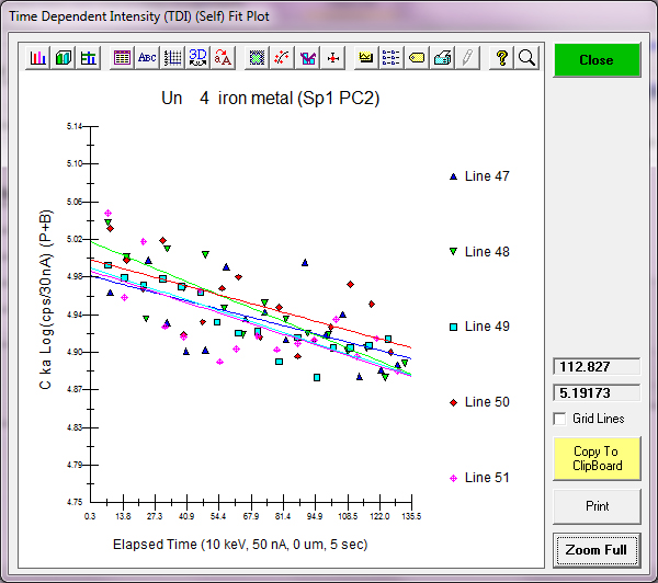
First of all, just as shown in the previously acquired data above, the carbon signal shows a small *decrease* over time while all other elements remain stable within precision:



Here is nitrogen Ka:



As for the quant, here you can see that results on a pure Fe std (but acquired separately from the MAN background stds), gives zero within precision for all elements (except for Si at 230 PPM which could be due to the colloidal Si polishing) :

Un    4 iron metal, Results in Elemental Weight Percents
 
ELEM:        C       N      Mo      Fe      Si
BGDS:      MAN     MAN     LIN     LIN     EXP
TIME:    80.00   80.00   60.00   60.00   60.00
BEAM:    49.75   49.75   49.75   49.75   49.75

ELEM:        C       N      Mo      Fe      Si   SUM 
    47   -.023   -.018   -.025 100.090    .023 100.047
    48    .032    .037    .005 100.471    .025 100.570
    49   -.010   -.043   -.006 101.030    .021 100.992
    50    .005    .006   -.004 100.380    .026 100.414
    51   -.013   -.030   -.031 100.456    .021 100.404

AVER:    -.002   -.010   -.012 100.486    .023 100.485
SDEV:     .021    .032    .015    .341    .002    .342
SERR:     .010    .014    .007    .152    .001
%RSD: -1244.94 -331.31 -125.84     .34   10.30
STDS:      506     672     542     526     514

STKF:    .9705   .1485   .9901  1.0000  1.0000
STCT:  23361.3   459.1  4349.2  1085.6 73411.0

UNKF:    .0000  -.0001  -.0001  1.0048   .0002
UNCT:      -.2     -.2     -.5  1090.8    15.0
UNBG:    148.0    13.6     9.2     7.9   134.1

ZCOR:   2.4870  1.5301  1.1661  1.0000  1.1457
KRAW:    .0000  -.0004  -.0001  1.0048   .0002
PKBG:     1.00     .99     .95  139.30    1.11
INT%:     ----    ----    ----    ----    ----

TDI%:    5.364   -.141    ----    ----    ----
DEV%:       .6     3.2    ----    ----    ----
TDIF:  LOG-LIN LOG-LIN    ----    ----    ----
TDIT:   131.80  134.00    ----    ----    ----
TDII:     148.    13.3    ----    ----    ----
TDIL:     5.00    2.59    ----    ----    ----


I also performed some "fast" beam scans in Probe Image *on the same spot* on pure Fe and will examine that data next week for TDI effects, but in the meantime here is my question:  is the small decrease in carbon signal over time, something that is observed on other instruments?

I would have thought that the carbon signal would increase over time, not decrease...   so I have to wonder if the cryo baffle (~100 Kelvin) on my instrument is somehow related to this?   I would be very grateful for similar measurement results by other labs...  thanks!

Again this is a freshly polished Fe metal sample coated with 15 nm Ag and measured at 10 keV and 50 nA. In any case, a standard deviation of around 200 PPM for carbon in 80 seconds isn't bad. That is, with a 5% TDI correction (+/- 0.6%). Which would correspond to an absolute TDI correction of ~800 +/- 100 PPM concentration.

Finally, is this decrease in carbon intensity simply related to the so called "decontamination time", as coined by Stuart Kearns, et al.

http://probesoftware.com/smf/index.php?topic=48.msg161#msg161

Though I would have expected the decontamination effect to apply only to the first 10 seconds or so, at most?

[Ben Buse]

Hi John,

I think its the decontamination effect as you mention. Your not hitting it that hard so its taking a long time to remove the surface carbon. What spot size did you use? I did some tests a while back - but I don't know where the TDI curves are. Anyway I decided at 100 nA 15kV 1um beam I wanted to hit the sample for ca, 30-60 secs before analyzing it. The TDI curves were variable in there behavior but generally over the first 30-60 secs the carbon decreased and then flattened. This was using a LN cold trap.

Have you tried the tdi for a longer time/different power - does it flatten our with time - suggestive of decomtamination?

What's your cryobuffer - is this a cold finger/trap?

It does seem complex as to the regime in which carbon contamination is being removed under the electron beam and when it is being deposited. Removal at high power, directly under the beam, depends on material - and therefore heating of sample, greatly aided by oxygen airjet/ deposition adjacent to the beam as a ring - but also sometimes under the beam.

There is also the issue of beam stability sometimes during the tdi the beam can drift onto the surrounding carbon ring giving a sharp rise.



Ben

[Probeman]

I think its the decontamination effect as you mention. Your not hitting it that hard so its taking a long time to remove the surface carbon. What spot size did you use? I did some tests a while back - but I don't know where the TDI curves are. Anyway I decided at 100 nA 15kV 1um beam I wanted to hit the sample for ca, 30-60 secs before analyzing it. The TDI curves were variable in there behavior but generally over the first 30-60 secs the carbon decreased and then flattened. This was using a LN cold trap.

Have you tried the tdi for a longer time/different power - does it flatten our with time - suggestive of decomtamination?

This was 10 keV, 50 nA fully focused.  I have to say I'm a little surprised that you think it might take 30-60 seconds to "de-contaminate", but I guess I could try with a less focused beam. 

Remember, this is *not* a carbon coated sample, it was freshly polished and coated with 15 nm of silver.  Are you sure it takes 30-60 seconds with a fully focused beam at 50 nA to remove 1 to 2 nm of native hydrocarbon?

What's your cryobuffer - is this a cold finger/trap?

It does seem complex as to the regime in which carbon contamination is being removed under the electron beam and when it is being deposited. Removal at high power, directly under the beam, depends on material - and therefore heating of sample, greatly aided by oxygen airjet/ deposition adjacent to the beam as a ring - but also sometimes under the beam.

There is also the issue of beam stability sometimes during the tdi the beam can drift onto the surrounding carbon ring giving a sharp rise.

We have a 100 Kelvin baffle over the diffusion pump, no air jet.  I know a carbon ring will form eventually, and when stage scanning, we see the carbon ring being intercepted effect as noted here:

http://probesoftware.com/smf/index.php?topic=114.msg3258#msg3258

Which is what we are trying to *avoid*, by scanning the beam over the analysis area.  I'll be posting that data later today, stay tuned!
john

[Probeman]

Here are my results (attached below) from performing 10 stage scans each 32 pixels wide (~4000x or ~94 um wide), using carbon Ka (and nitrogen Ka) on pure Fe (freshly polished and coated with 15 nm of Ag), with each scan repeated on the same area.

The 10 stage scans were separately defined in Probe Image (actually pretty easy to do, but I will have Brian implement a TDI option if this method turns out to be as promising as it seems to look), and therefore each scan took about 32 seconds of actual acquisition time and around 45 seconds each with all the software/hardware overhead involved. 

Of course I will also need to modify CalcImage so it automatically loads in these replicate TDI scans so it can extrapolate automatically back to zero time, but that shouldn't be too difficult as Probe Image already time stamps each scan at the beginning and end automatically.  This should work whether the scan is a line scan or a full frame scan...

The total time on each pixel was about 10 seconds, which is what we would likely utilize for trace carbon analyses although of course this could be increased for improved sensitivity.

I have to say this method might be very useful for trace carbon analyses, not to mention beam sensitive samples!   Has anyone heard of this idea previously?  Or tried it yourself?

[JohnF]

Having done with Phil here earlier today a C Ka TDI count, I have a comment/suggestion.
A TDI acquisition was done (spot mode) so we aren't talking imaging, but rather the philosophy of TDI upon 'sensitive' material, and we did a similar acquisition and it showed a 'linear' (in the log window).
I was suspicious, so said, instead of having a LONNNGGG dwell period of 12 seconds, let's be devils advocates and see if, like in hydrous alkali glasses, whether there is an immediate change in the first second or so...and guess what, the plot now was exponential on the log window.

We were going to suggest that you might want to implement a modified TDI approach, in allowing the user to pick an option of doing a (variable short time, such as one second)) count for the _first_ measurement, which could pick up any sharp change over the first count period.

I know it might be difficult to implement, but you are a smart guy!

[Probeman]

Having done with Phil here earlier today a C Ka TDI count, I have a comment/suggestion.
A TDI acquisition was done (spot mode) so we aren't talking imaging, but rather the philosophy of TDI upon 'sensitive' material, and we did a similar acquisition and it showed a 'linear' (in the log window).
I was suspicious, so said, instead of having a LONNNGGG dwell period of 12 seconds, let's be devils advocates and see if, like in hydrous alkali glasses, whether there is an immediate change in the first second or so...and guess what, the plot now was exponential on the log window.

We were going to suggest that you might want to implement a modified TDI approach, in allowing the user to pick an option of doing a (variable short time, such as one second)) count for the _first_ measurement, which could pick up any sharp change over the first count period.

I know it might be difficult to implement, but you are a smart guy!

Flattery will get you everywhere!     

Seriously, this would be pretty difficult to implement.  You do know about the option where one can weight the first few TDI measurements?

http://probesoftware.com/smf/index.php?topic=11.msg2520#msg2520

It sort of amounts to the same thing you and Phil are suggesting...

By the way, here are the N Ka data that was acquired at the same time (see attached below). The confidence intervals displayed are for 99%.

Again, by the way, these analyses were performed *without* a blank correction, which would obviously improve these trace measurements.

[John Donovan]

I would sum up by saying that one can perform excellent trace carbon quantitative analyses using the following methods together:

1. MAN backgrounds

2. Normal matrix corrections

3. Quantitative interference corrections (a la PFE)

4. TDI correction (I generally use asynchronous mode as the new acquisition code doesn't really take any longer than the old synchronous code).

Remember, if you have a suitable standard with a matching matrix, one can alternatively perform a "blank" correction, but not with the interference correction, or you will get a "double" correction on the trace element... though the software will warn you about this!