I think it would be a good idea to take this Ti in quartz discussion in a step by step fashion because it is all rather complicated at first.
So we'll start by acquiring Ti Ka on all 5 spectrometers. We'll get the best detection limits using the PET crystal variety, but this measurement could also be done on all LIF crystals or a mixture of PET and LIF Bragg crystals as long as the standards and unknowns are acquired using the same sample setup (which is the default mode in PFE).
On our instrument we used this setup and acquired in this case 960 seconds on-peak and the same amount of time off-peak. That's over half an hour which is a fairly long time, especially since it is well known that quartz crystal (in contrast to quartz glass) is visibly damaged by the electron beam. Particularly since we are using a 200 nA beam current!
To minimize the effect of prolonged exposure of the beam on the quartz we utilize the "alternating on and off peak" acquisition method. This method is activated by a single mouse click to one's sample setup in the Acquisition Option dialog from the Acquire! window as seen here (note that Ti Ka on an PET crystal is specified for each spectrometer):
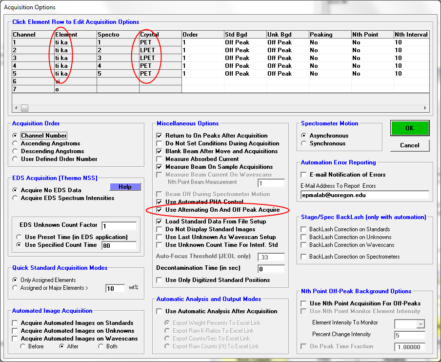
What this does is break up the acquisition into a number of cycles that "alternates" between on-peak and off-peak measurements. We can specify the number of cycles utilized using the "Unknown Count Factor" parameter in the Count Times dialog. Since we are counting all the elements the same way, we can simply click and drag all five element rows in the Count Times dialog and then we will see this dialog for the "Selected Elements":
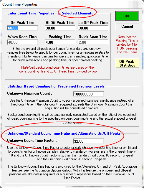
By specifying an Unknown Count Factor for all the Ti channels, we are telling the software to alternate between the on and off peak measurements 32 times per data point acquisition. This interval data is saved automatically and can be plotted as seen here where we can see a small but consistent downwards trend in the background corrected intensities.

The point being that the "delta" between the peak and off-peak is being tracked over time for the most reliable measurement. When this is done we can see the resulting quantitative analysis performed on an SiO2 "blank" standard, which has been previously characterized by ICP-MS as containing 1.42 PPM Ti, as seen in this output:
Un 30 960 sec on SiO2
TakeOff = 40.0 KiloVolt = 20.0 Beam Current = 200. Beam Size = 20
(Magnification (analytical) = 8000), Beam Mode = Analog Spot
(Magnification (default) = 600, Magnification (imaging) = 100)
Image Shift (X,Y): .00, .00
Number of Data Lines: 5 Number of 'Good' Data Lines: 5
First/Last Date-Time: 06/12/2009 04:58:27 PM to 06/12/2009 07:26:32 PM
WARNING- Using Alternating On and Off Peak Acquisition
Average Total Oxygen: 53.255 Average Total Weight%: 99.994
Average Calculated Oxygen: 53.255 Average Atomic Number: 10.804
Average Excess Oxygen: .000 Average Atomic Weight: 20.028
Average ZAF Iteration: 1.00 Average Quant Iterate: 2.00
Oxygen Calculated by Cation Stoichiometry and Included in the Matrix Correction
WARNING- Duplicate analyzed elements are present in the sample matrix!!
Use Aggregate Intensity option or Disable Quant feature for accurate matrix correction.
Un 30 960 sec on SiO2, Results in Elemental Weight Percents
ELEM: Ti Ti Ti Ti Ti Si O
TYPE: ANAL ANAL ANAL ANAL ANAL SPEC CALC
BGDS: LIN LIN LIN LIN LIN
TIME: 960.00 960.00 960.00 960.00 960.00
BEAM: 199.56 199.56 199.56 199.56 199.56
ELEM: Ti Ti Ti Ti Ti Si O SUM
XRAY: (ka) (ka) (ka) (ka) (ka) () ()
266 -.00015 -.00116 -.00256 .00003 -.00006 46.7430 53.2544 99.9935
267 .00076 -.00160 -.00336 .00081 -.00006 46.7430 53.2547 99.9943
268 -.00013 -.00104 -.00324 .00038 -.00002 46.7430 53.2543 99.9932
269 .00026 -.00101 -.00302 .00124 -.00035 46.7430 53.2551 99.9952
270 -.00011 -.00090 -.00265 .00119 -.00022 46.7430 53.2552 99.9955
AVER: .00012 -.00114 -.00297 .00073 -.00014 46.743 53.255 99.9943
SDEV: .00039 .00027 .00035 .00052 .00014 .000 .000 .00100
SERR: .00018 .00012 .00016 .00023 .00006 .00000 .00018
%RSD: 317.644 -23.837 -11.885 71.4915 -97.829 .00000 .00076
STDS: 922 922 922 922 922 0 0
STKF: .5883 .5883 .5883 .5883 .5883 .0000 .0000
STCT: 667.34 1600.07 1901.70 531.93 828.32 .00 .00
UNKF: .0000 .0000 .0000 .0000 .0000 .0000 .0000
UNCT: .00 -.03 -.08 .01 .00 .00 .00
UNBG: .99 2.64 3.42 .79 1.38 .00 .00
ZCOR: 1.1969 1.1969 1.1969 1.1969 1.1969 .0000 .0000
KRAW: .00000 -.00002 -.00004 .00001 .00000 .00000 .00000
PKBG: 1.00119 .99017 .97657 1.00705 .99878 .00000 .00000
Detection limit at 99 % Confidence in Elemental Weight Percent (Single Line):
ELEM: Ti Ti Ti Ti Ti
266 .00072 .00049 .00047 .00081 .00068
267 .00072 .00049 .00047 .00081 .00069
268 .00072 .00049 .00047 .00081 .00069
269 .00072 .00049 .00047 .00080 .00068
270 .00072 .00049 .00047 .00080 .00068
AVER: .00072 .00049 .00047 .00080 .00068
SDEV: .00000 .00000 .00000 .00000 .00000
SERR: .00000 .00000 .00000 .00000 .00000From the calculated detection limits just above we can see that we are getting quite reasonable detection limits from 0.00047 wt.% (4.7 PPM) to 0.0008 wt.% (8 PPM) so what could we possibly complain about? Well, for one thing, our average concentrations (AVER:) are *larger* from zero (1.42 PPM) than our standard deviations! This means that we have better precision now than accuracy. That is to say we cannot accurately measure zero (1.42 PPM) as well as our sensitivity.
For example, on spectrometer 2 we have a standard deviation of 0.00027 (2.7 PPM) and a quantitative result of 0.00114 (11.4 PPM). Even with 3 sigma statistics we cannot reconcile that, so we have an accuracy problem. Spectrometer 3 shows an even larger accuracy issue.
What is causing that? Well take a look at this slide and we can see that this could be caused by several different factors. But since these are Ti in SiO2 measurements on a PET crystal we know that the "holes" in the continuum can be caused by secondary Bragg diffraction of the PET crystal.
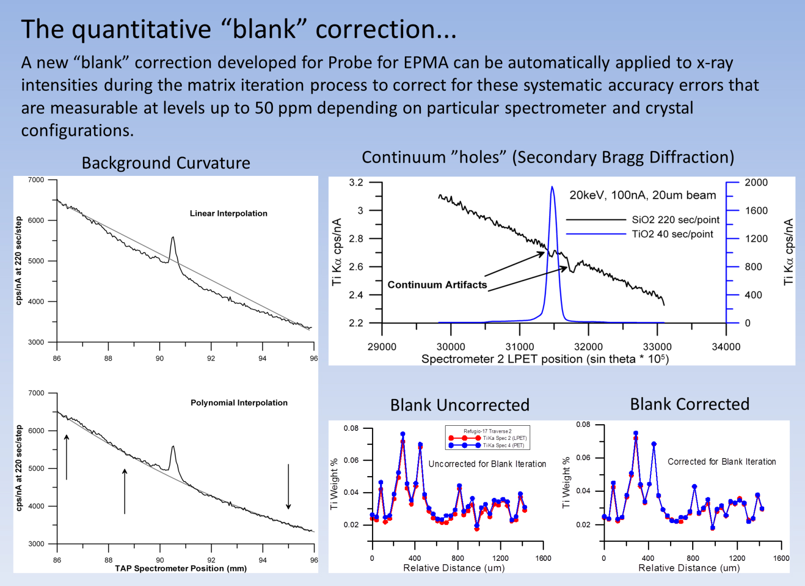
The hole in the Ti continuum to the right side of the peak can be avoided, but *not* the smaller hole in the background which is right underneath the Ti Ka peak!
But the point is that we can already make a correction for these continuum artifacts since we have characterized an SiO2 standard containing a zero or known (in this case 1.42 PPM) amount of Ti in SiO2. To illustrate this we will perform an analysis of the same sample, but this time using the intensities from a previous 960 second acquisition as a "blank" correction which is done simply by selecting the sample in the Standard Assignments dialog as seen here:
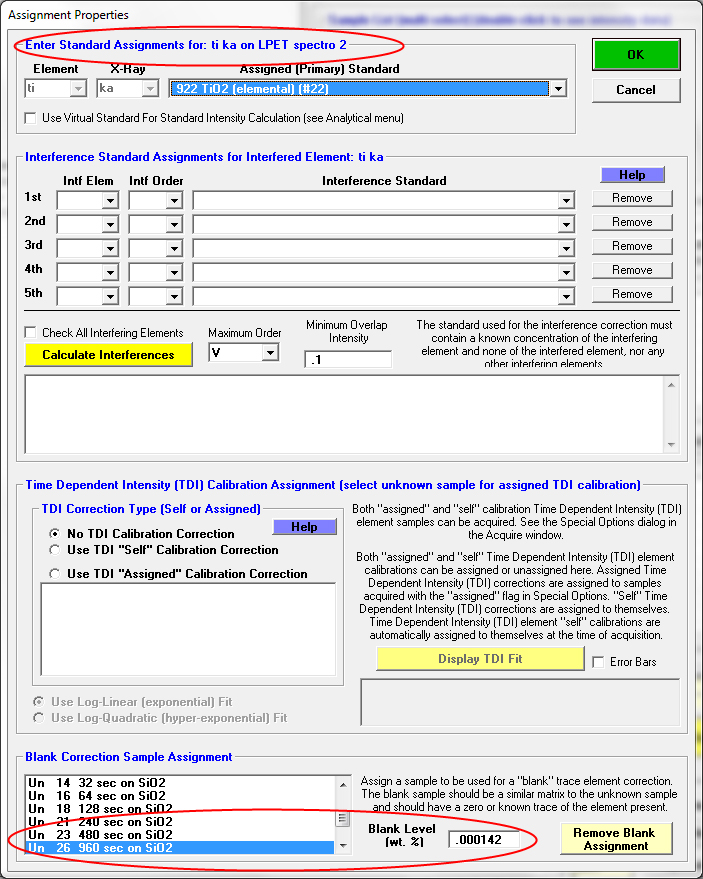
Note that the blank assignment needs to be specified for each Ti channel (note that we specified 0.000142 (1.42 PPM) as the "blank" level, but we could also have just left the default as zero since the Ti level is so close to zero). Once that is done, we can re-calculate our test sample and we now get the following "blank" corrected results:
Un 30 960 sec on SiO2
TakeOff = 40.0 KiloVolt = 20.0 Beam Current = 200. Beam Size = 20
(Magnification (analytical) = 8000), Beam Mode = Analog Spot
(Magnification (default) = 600, Magnification (imaging) = 100)
Image Shift (X,Y): .00, .00
Number of Data Lines: 5 Number of 'Good' Data Lines: 5
First/Last Date-Time: 06/12/2009 04:58:27 PM to 06/12/2009 07:26:32 PM
WARNING- Using Blank Trace Correction
WARNING- Using Alternating On and Off Peak Acquisition
Average Total Oxygen: 53.258 Average Total Weight%: 100.002
Average Calculated Oxygen: 53.258 Average Atomic Number: 10.805
Average Excess Oxygen: .000 Average Atomic Weight: 20.029
Average ZAF Iteration: 1.00 Average Quant Iterate: 3.00
Oxygen Calculated by Cation Stoichiometry and Included in the Matrix Correction
WARNING- Duplicate analyzed elements are present in the sample matrix!!
Use Aggregate Intensity option or Disable Quant feature for accurate matrix correction.
Un 30 960 sec on SiO2, Results in Elemental Weight Percents
ELEM: Ti Ti Ti Ti Ti Si O
TYPE: ANAL ANAL ANAL ANAL ANAL SPEC CALC
BGDS: LIN LIN LIN LIN LIN
TIME: 960.00 960.00 960.00 960.00 960.00
BEAM: 199.56 199.56 199.56 199.56 199.56
ELEM: Ti Ti Ti Ti Ti Si O SUM
XRAY: (ka) (ka) (ka) (ka) (ka) () ()
266 .00007 .00022 .00053 -.00030 .00042 46.7430 53.2576 100.002
267 .00098 -.00023 -.00027 .00049 .00043 46.7430 53.2579 100.002
268 .00010 .00033 -.00015 .00005 .00046 46.7430 53.2575 100.001
269 .00048 .00037 .00007 .00091 .00013 46.7430 53.2583 100.003
270 .00011 .00047 .00044 .00086 .00026 46.7430 53.2584 100.004
AVER: .00035 .00023 .00012 .00040 .00034 46.743 53.258 100.002
SDEV: .00039 .00027 .00035 .00052 .00014 .000 .000 .00100
SERR: .00018 .00012 .00016 .00023 .00006 .00000 .00018
%RSD: 112.699 117.296 291.993 129.733 41.2622 .00000 .00075
STDS: 922 922 922 922 922 0 0
STKF: .5883 .5883 .5883 .5883 .5883 .0000 .0000
STCT: 667.34 1600.07 1901.70 531.93 828.32 .00 .00
UNKF: .0000 .0000 .0000 .0000 .0000 .0000 .0000
UNCT: .00 .01 .00 .00 .00 .00 .00
UNBG: .99 2.64 3.42 .79 1.38 .00 .00
ZCOR: 1.1969 1.1969 1.1969 1.1969 1.1969 .0000 .0000
KRAW: .00000 .00000 .00000 .00001 .00000 .00000 .00000
PKBG: 1.00333 1.00200 1.00096 1.00389 1.00290 .00000 .00000
BLNK#: 26 26 26 26 26 ---- ----
BLNKL: .000142 .000142 .000142 .000142 .000142 ---- ----
BLNKV: -.00008 -.00123 -.00295 .000471 -.00034 ---- ----[/tt]
Note the lines in red color which show the sample assigned as the "blank" correction, the "blank" level (1.42 PPM) and the "blank" value, which is the concentration by which our measurement differs from the known concentration of Ti in our blank standard. Note that spectrometer 3 has a continuum artifact of 0.00295 wt.% (~30 PPM)!
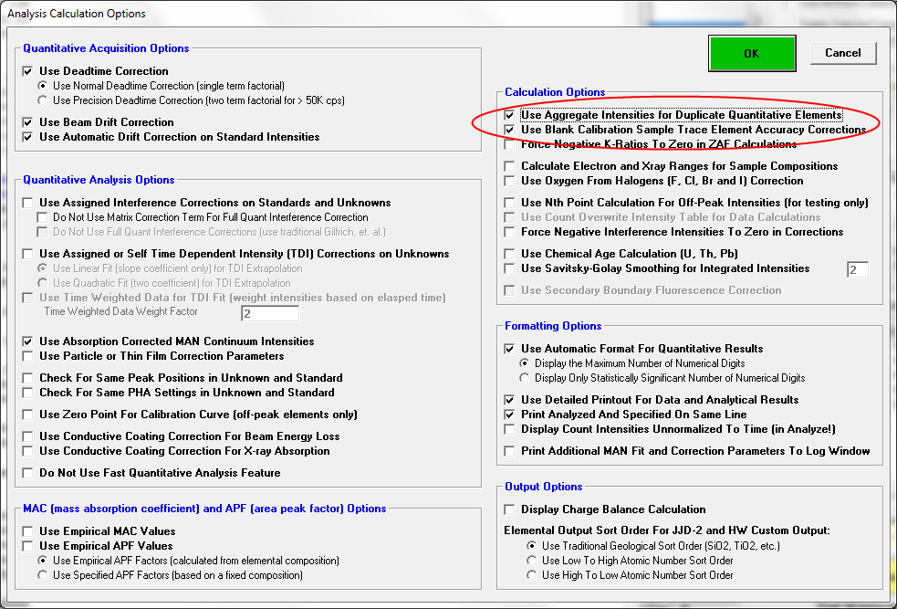
Now we can see that our accuracy is similar to our precision in the AVER: and SDEV: lines above around 4 to 5 PPM. So now can we further improve our statistics by increasing our geometric efficiency? Yes, by "aggregating" our 5 spectrometers into a single "giant virtual" spectrometer. We'll have to aggregate the photons for both our on-peak and off-peak intensities and also for both the standard and unknown (and also of course the blank standard as well).
When we do this, by simply clicking the checkbox seen here (which also shows how every software correction we have specified can be globally turned on or off *without* changing the actual sample assignments for quick comparisons):
we obtain the following results:
Un 30 960 sec on SiO2
TakeOff = 40.0 KiloVolt = 20.0 Beam Current = 200. Beam Size = 20
(Magnification (analytical) = 8000), Beam Mode = Analog Spot
(Magnification (default) = 600, Magnification (imaging) = 100)
Image Shift (X,Y): .00, .00
Number of Data Lines: 5 Number of 'Good' Data Lines: 5
First/Last Date-Time: 06/12/2009 04:58:27 PM to 06/12/2009 07:26:32 PM
WARNING- Using Blank Trace Correction
WARNING- Using Alternating On and Off Peak Acquisition
WARNING- Using Aggregate Intensities for Duplicate Elements
Average Total Oxygen: 53.257 Average Total Weight%: 100.000
Average Calculated Oxygen: 53.257 Average Atomic Number: 10.805
Average Excess Oxygen: .000 Average Atomic Weight: 20.029
Average ZAF Iteration: 1.00 Average Quant Iterate: 3.00
Oxygen Calculated by Cation Stoichiometry and Included in the Matrix Correction
Un 30 960 sec on SiO2, Results in Elemental Weight Percents
ELEM: Ti Ti Ti Ti Ti Si O
TYPE: ANAL ANAL ANAL ANAL ANAL SPEC CALC
BGDS: LIN LIN LIN LIN LIN
TIME: 960.00 .00 .00 .00 .00
BEAM: 199.56 .00 .00 .00 .00
AGGR: 5
ELEM: Ti Ti Ti Ti Ti Si O SUM
XRAY: (ka) (ka) (ka) (ka) (ka) () ()
266 .00028 .00000 .00000 .00000 .00000 46.7430 53.2572 100.001
267 .00007 .00000 .00000 .00000 .00000 46.7430 53.2571 100.000
268 .00013 .00000 .00000 .00000 .00000 46.7430 53.2571 100.000
269 .00029 .00000 .00000 .00000 .00000 46.7430 53.2572 100.001
270 .00041 .00000 .00000 .00000 .00000 46.7430 53.2573 100.001
AVER: .00024 .00000 .00000 .00000 .00000 46.743 53.257 100.000
SDEV: .00014 .00000 .00000 .00000 .00000 .000 .000 .00023
SERR: .00006 .00000 .00000 .00000 .00000 .00000 .00004
%RSD: 57.1257 .00002 .00002 .00002 .00002 .00000 .00017
STDS: 922 0 0 0 0 0 0
STKF: .5621 .0000 .0000 .0000 .0000 .0000 .0000
STCT: 5529.37 .00 .00 .00 .00 .00 .00
UNKF: .0000 .0000 .0000 .0000 .0000 .0000 .0000
UNCT: .02 .00 .00 .00 .00 .00 .00
UNBG: 9.23 .00 .00 .00 .00 .00 .00
ZCOR: 1.1969 .0000 .0000 .0000 .0000 .0000 .0000
KRAW: .00000 .00000 .00000 .00000 .00000 .00000 .00000
PKBG: 1.00211 .00000 .00000 .00000 .00000 .00000 .00000
BLNK#: 26 26 26 26 26 ---- ----
BLNKL: .000142 .000142 .000142 .000142 .000142 ---- ----
BLNKV: -.00133 .000000 .000000 .000000 .000000 ---- ----Wow! We got 2.4 PPM +/- 1.4 PPM or less than one sigma within our blank standard of 1.42 PPM Ti.
Please refer to this publication which describes these methods in more detail:
http://probesoftware.com/Ti%20in%20Quartz,%20Am.%20Min.%20Donovan,%202011.pdfNext a look at t-testing for confidence- after all we *only* acquired 5 data points in our average not an infinite number!


 Remember, you need to be logged in to see posted attachments!